लोचदार स्थैतिक विश्लेषण के वास्तविक मॉडल उदाहरण

विश्लेषण मॉडल

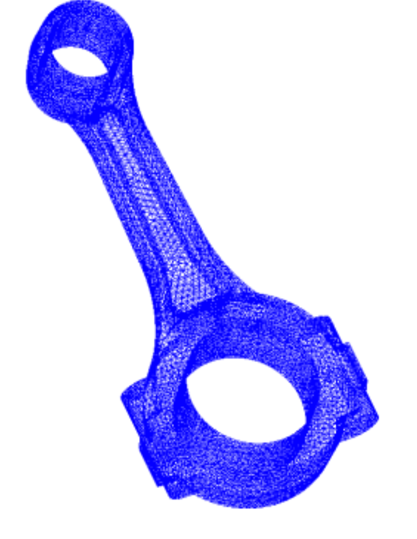
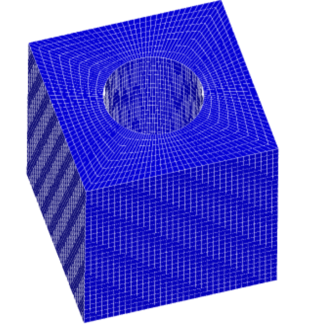
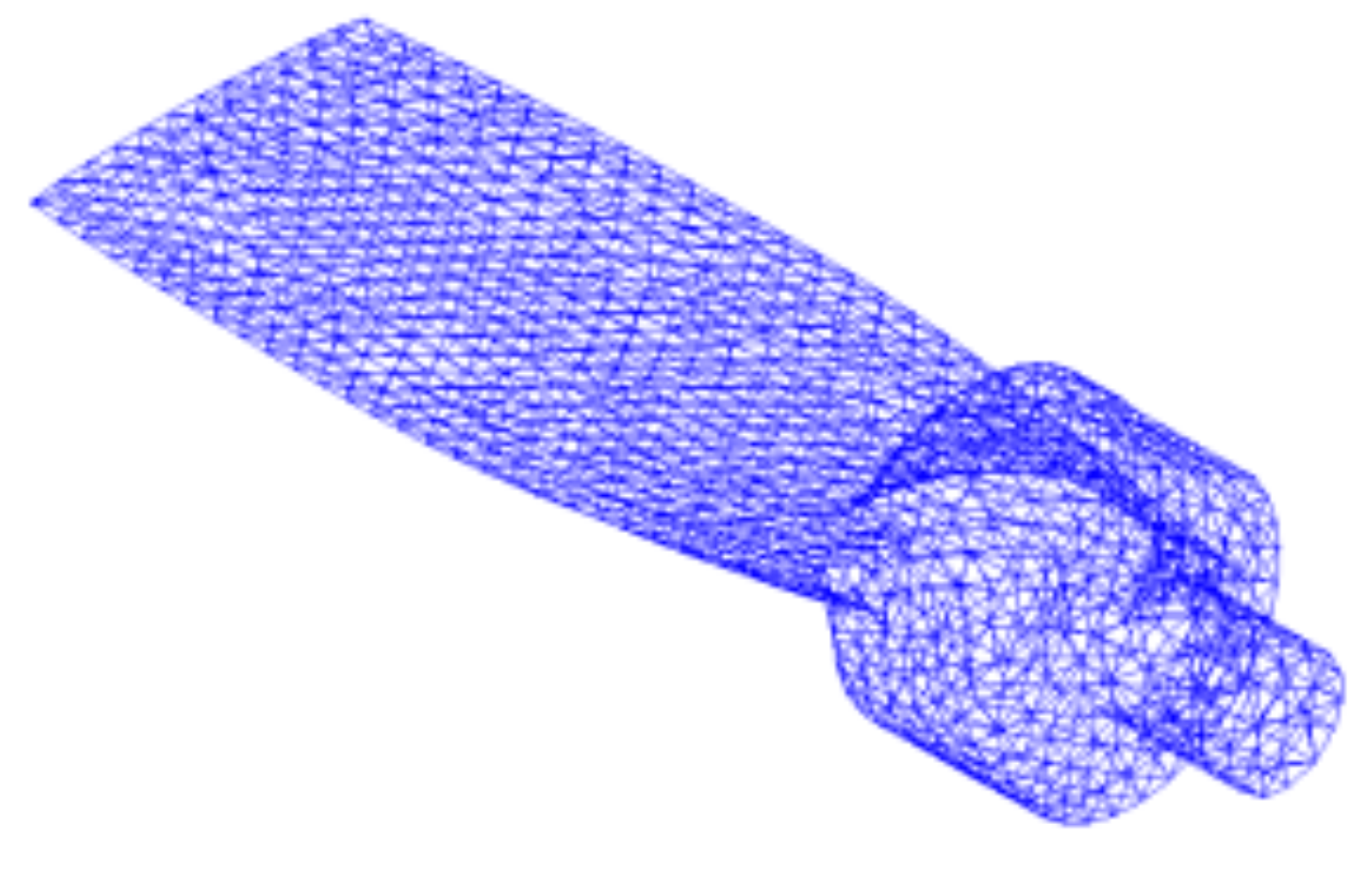
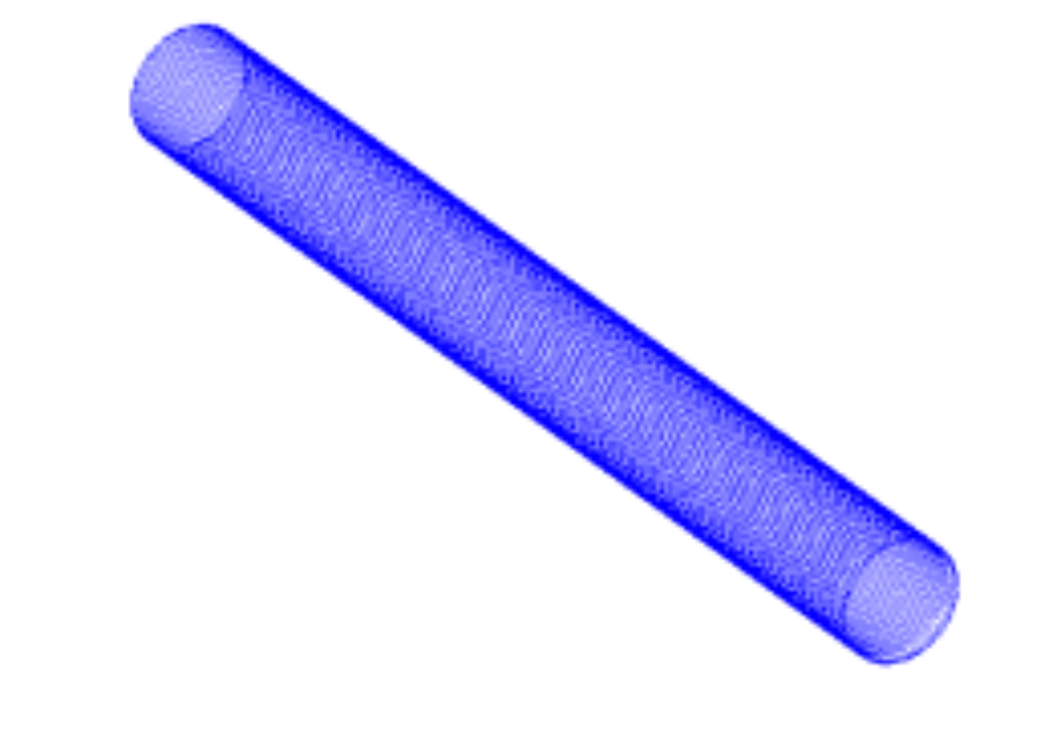
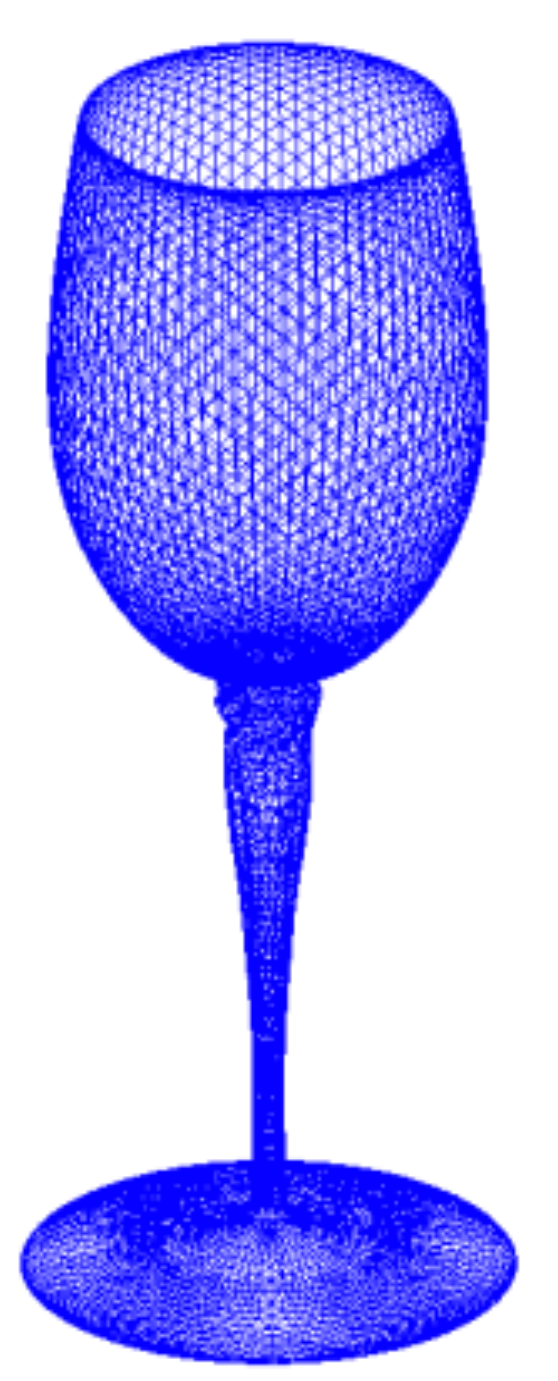
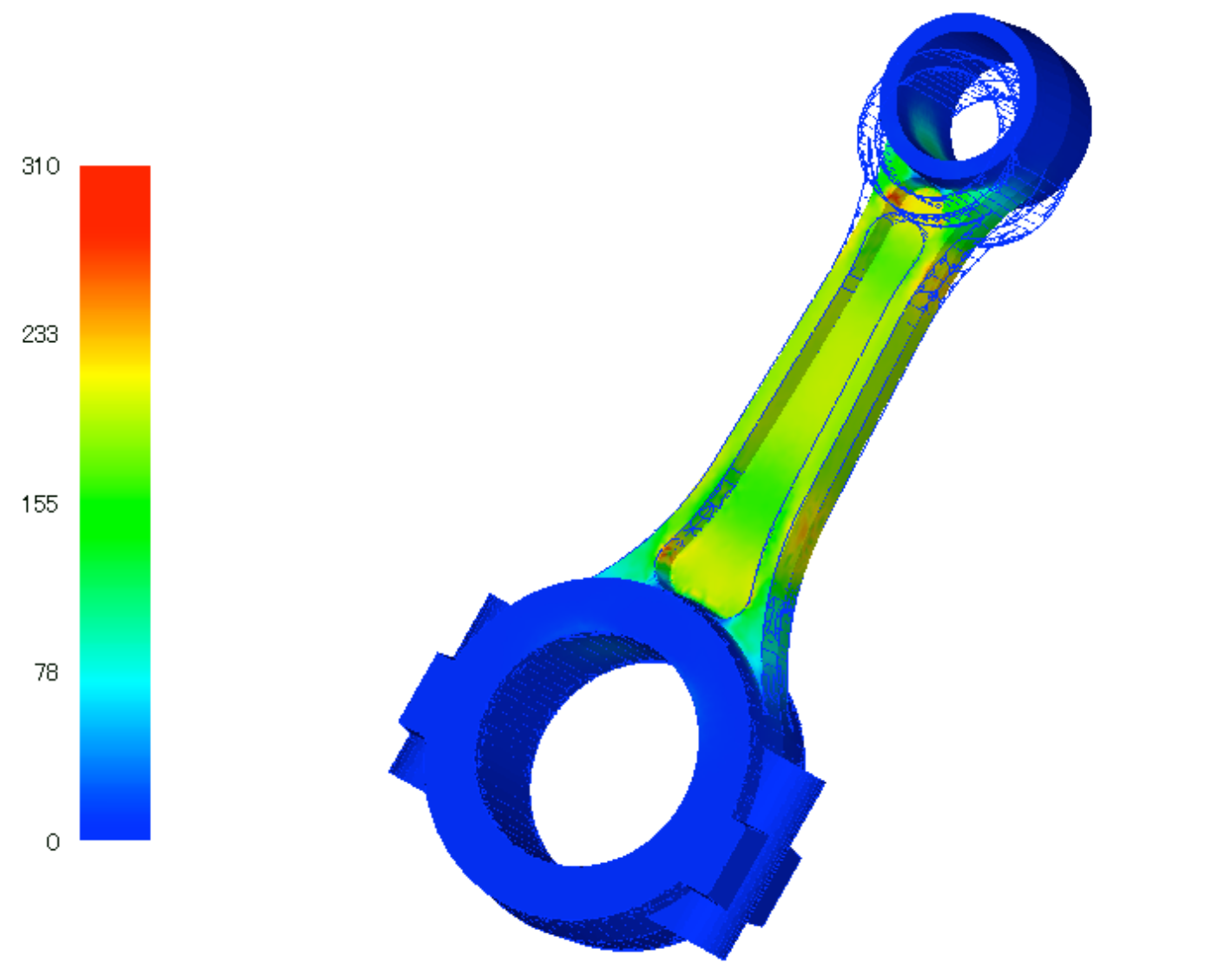
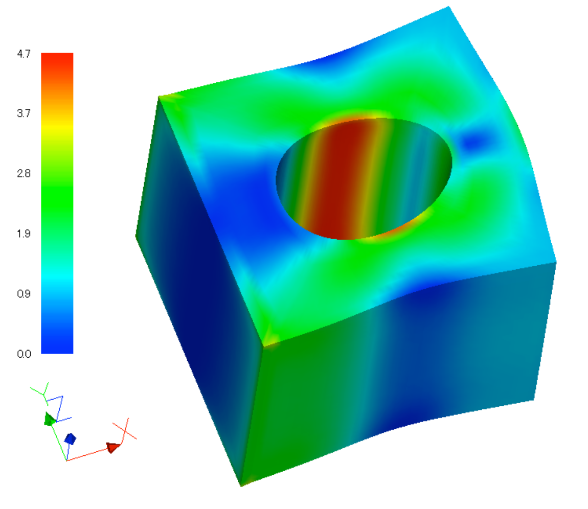
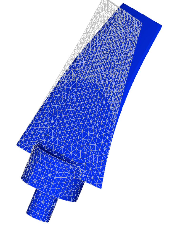
तालिका 9.2.1 लोचदार स्थैतिक विश्लेषण के actual-model verification examples सूचीबद्ध करती है। कुछ अपवादों को छोड़कर models के shapes चित्र 9.2.1 से 9.2.5 में भी दिखाए गए हैं। element types 731 और 741 वाले examples चलाने के लिए अलग direct solver आवश्यक है।

तालिका 9.2.1 लोचदार स्थैतिक विश्लेषण के वास्तविक मॉडल verification examples

केस नाम	तत्व प्रकार	verification model	नोडों की संख्या	स्वतंत्रता डिग्रियाँ
EX01A	342	Connecting rod (100,000 nodes)	94,074	282,222
EX01B	342	Connecting rod (330,000 nodes)	331,142	993,426
EX02	361	छिद्र वाला block	37,386	112,158
EX03	342	Turbine blade	10,095	30,285
EX04	741	Cylindrical shell	10,100	60,600
EX05A	731	Wine glass (coarse)	7,240	43,440
EX05B	731	Wine glass (medium)	48,803	292,818
EX05C	731	Wine glass (fine)	100,602	603,612

चित्र 9.2.1 Connecting rod (EX01A)

चित्र 9.2.2 छिद्र वाला block (EX02)

चित्र 9.2.3 Turbine blade (EX03, EX06)

चित्र 9.2.4 Cylindrical shell (EX04, EX09)

चित्र 9.2.5 Wine glass (EX05, EX10A)

विश्लेषण परिणाम

उदाहरण विश्लेषण परिणाम

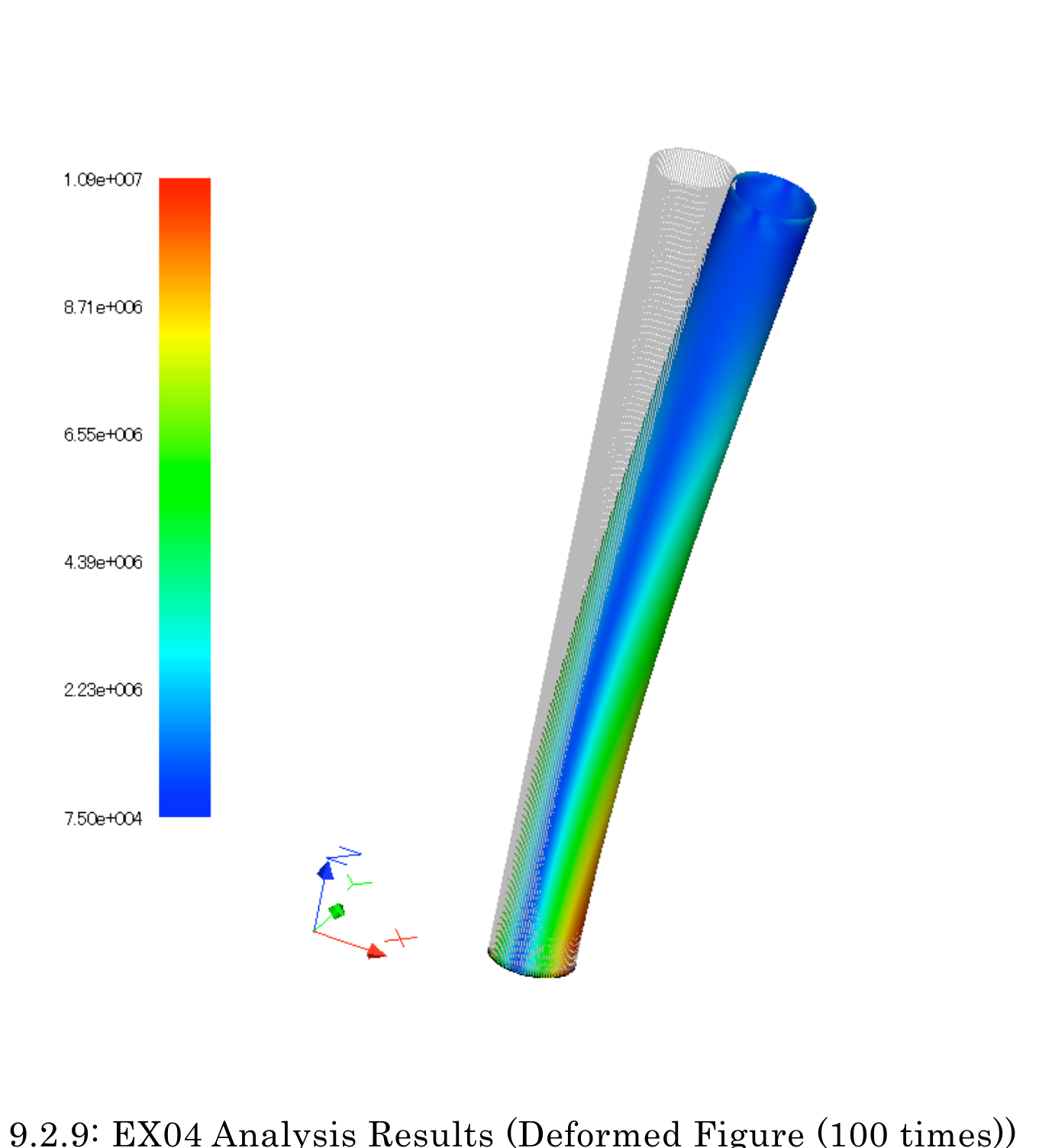
विश्लेषण परिणामों के उदाहरण चित्र 9.2.6 से 9.2.9 में दिखाए गए हैं।

चित्र 9.2.6 EX01A विश्लेषण परिणाम (Mises stress और deformation plot (10x))

चित्र 9.2.7 EX02 विश्लेषण परिणाम (Mises stress और deformation plot (100x))

चित्र 9.2.8 EX03 विश्लेषण परिणाम (deformation plot (10x))

चित्र 9.2.9 EX04 विश्लेषण परिणाम (deformation plot (100x))

उदाहरण EX02 का उपयोग करके विश्लेषण प्रदर्शन के सत्यापन परिणाम

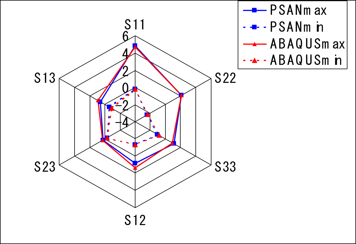
EX02 block-with-hole verification model के समतुल्य model का उपयोग करके general-purpose commercial software से analysis किया गया। चित्र 9.2.10 FrontISTR के मानों के साथ maximum और minimum stress-component values की तुलना दिखाता है। चित्र दिखाता है कि stress components बहुत निकटता से मेल खाते हैं।

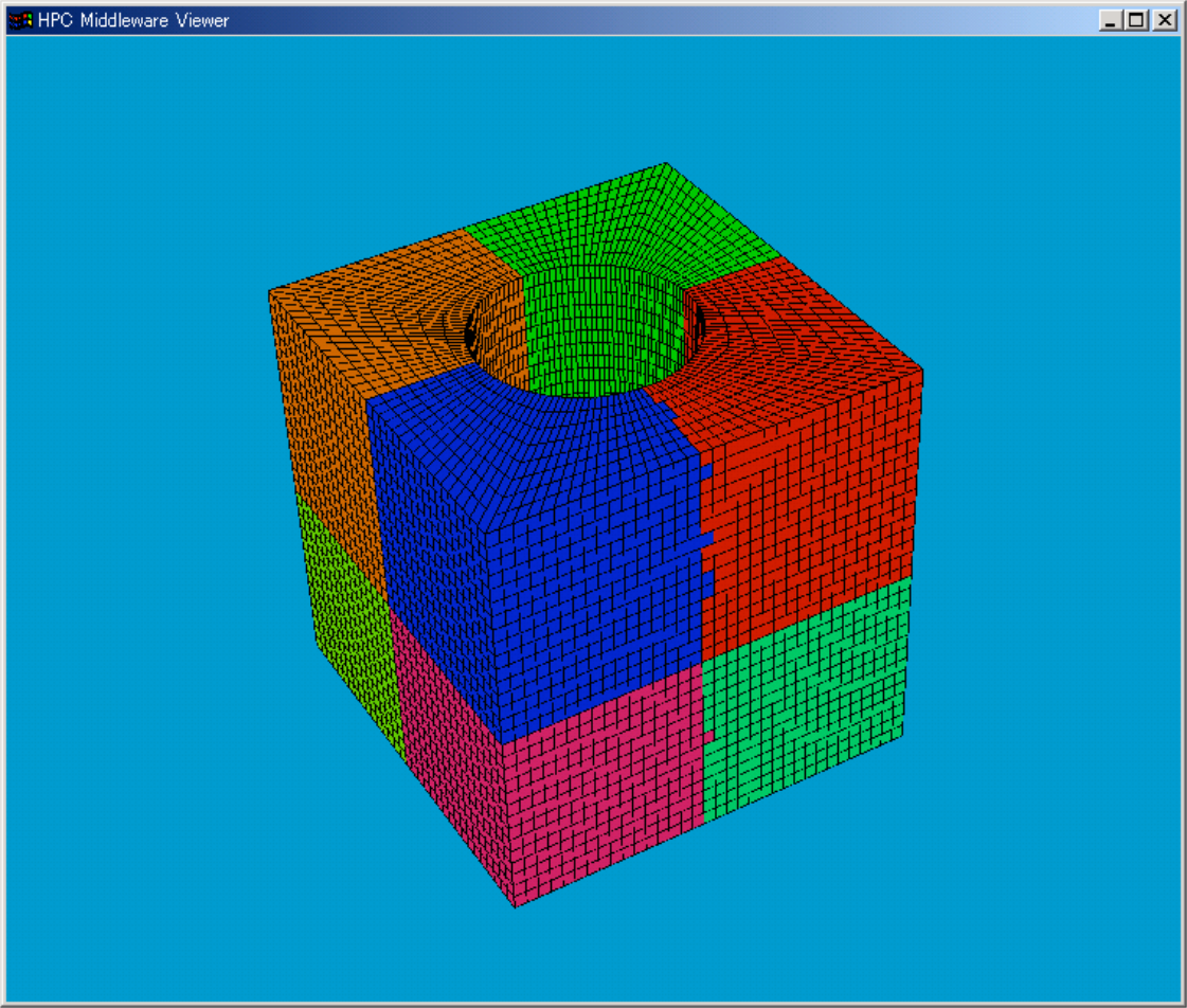
इसके बाद stress distribution पर domain partitioning के प्रभाव की जाँच की गई। RCB method का उपयोग करके domain partitioning किया गया, model को X, Y और Z प्रत्येक दिशा में दो भागों में बाँटकर कुल आठ domains बनाए गए। चित्र 9.2.11 partitioning दिखाता है। चित्र 9.2.12 single domain और आठ partitioned domains वाले analyses से प्राप्त stress distributions दिखाता है।

चित्र 9.2.10 EX02 में stress components की general-purpose software से तुलना

चित्र 9.2.11 RCB method से आठ domains में partition किया गया EX02

चित्र 9.2.12 domain partitioning के कारण Mises stress distribution में अंतर

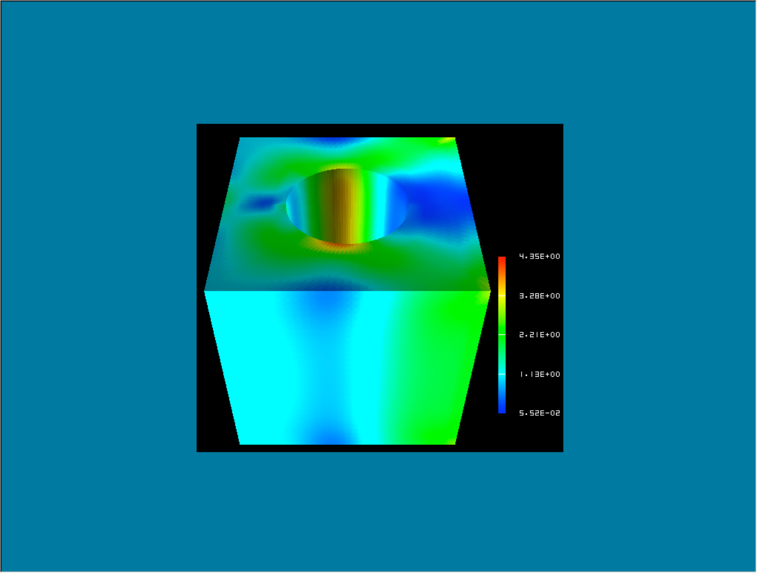
चित्र 9.2.12 दोनों results के बीच कोई अंतर नहीं दिखाता; वे पूर्णतः मेल खाते हैं।

तालिका 9.2.2 उपयोग किए गए HEC-MW solver settings के execution times की तुलना करती है। चित्र 9.2.13 solution तक की convergence history भी दिखाता है।

तालिका 9.2.2 HEC-MW solvers का उपयोग करते हुए execution times की तुलना

सॉल्वर	निष्पादन समय (s)
CGI	38.79
CGscale	52.75
BCGS	60.79
CG8	6.65

चित्र 9.2.13 HEC-MW solvers का उपयोग करते हुए convergence histories की तुलना (convergence threshold: 1.0x10^-8^)

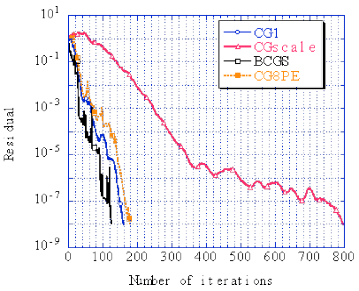
सत्यापन उदाहरण EX01A का उपयोग करके गणना समय की तुलना

verification example EX01A (connecting rod) का उपयोग करके domain partitioning से calculation में speedup का मूल्यांकन किया गया। calculation के लिए Xeon 2.8 GHz processors वाला 24-node cluster computer उपयोग किया गया। results चित्र 9.2.14 में दिखाए गए हैं। चित्र दिखाता है कि calculation speed domains की संख्या के अनुपात में बढ़ती है।

computer environment के कारण calculation time में अंतर की भी जाँच की गई। results तालिका 9.2.3 में दिखाए गए हैं।

चित्र 9.2.14 domain partitioning का speedup effect

तालिका 9.2.3 computer के अनुसार calculation times की तुलना (1 CPU)

CPU	Frequency [GHz]	OS	CPU Time [sec]	solver time [sec]
Xeon	2.8	Linux	850	817
Pentium III	0.866	Win2000	2008	1980
Pentium M	0.760	WinXP	1096	1070
Pentium 4	2.0	WinXP	802	785
Pentium 4	2.8	WinXP	738	718
Celeron	0.700	Win2000	2252	2215
Pentium 4	2.4	WinXP	830	804