Verification Using Simple-Geometry Models
Elastic Static Analysis
This verification uses a cantilever beam meshed as shown in Figure 9.1.1. Seven cases, exA through exG, were analyzed using the loading conditions shown in Figure 9.1.2. Case exG uses the same loading conditions as exA, but with a direct solver.
Verification results for each loading condition are shown in Tables 9.1.1 through 9.1.7.
 Figure 9.1.1 Example of a Cantilever-Beam Mesh (Hexahedral Elements)
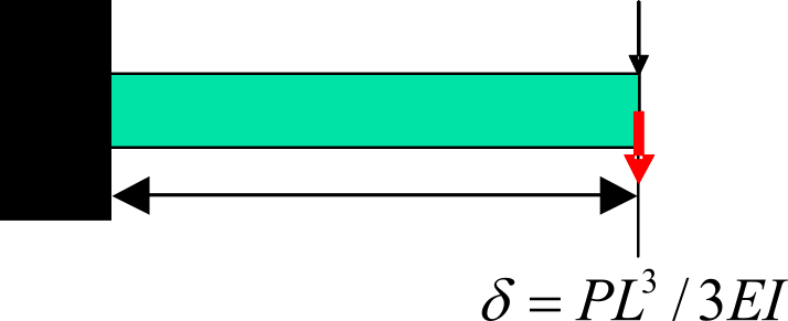 | (a) exA and exG: Concentrated load |
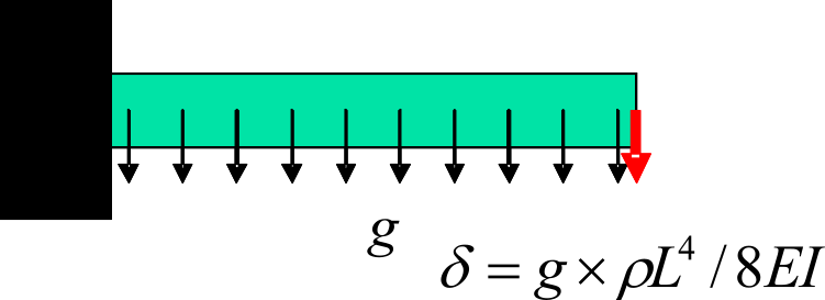 | (b) exD: Gravitational load |
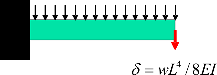 | (c) exB: Distributed surface load |
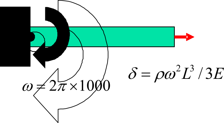 | (d) exE: Centrifugal force |
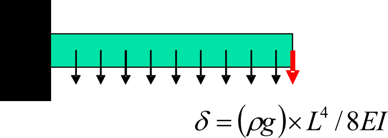 | (e) exC: Body load |
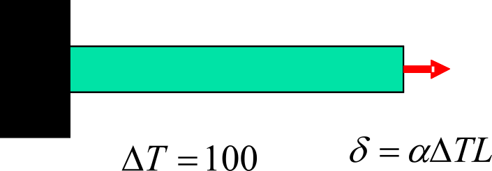 | (f) exF: Thermal load |
| Item | Value |
|---|---|
| Young's modulus | \(E = 4000.0\ \mathrm{kgf/mm^2}\) |
| Length | \(L = 10.0\ \mathrm{mm}\) |
| Poisson's ratio | \(\nu = 0.3\) |
| Cross-sectional area | \(A = 1.0\ \mathrm{mm^2}\) |
| Mass density | \(\rho = 8.0102 \times 10^{-10}\ \mathrm{kgf}\;\mathrm{s}^2/\mathrm{mm}^4\) |
| Second moment of area | \(I = 1.0/12.0\ \mathrm{mm^4}\) |
| Gravitational acceleration | \(g = 9800.0\ \mathrm{mm/s^2}\) |
| Coefficient of linear thermal expansion | \(\alpha = 1.0 \times 10^{-5}\) |
Figure 9.1.2 Verification Conditions for the Cantilever-Beam Model
Table 9.1.1 exA: Verification Results for the Concentrated-Load Problem
| Case Name | Number of Elements | Predicted Value: \(\delta_{max}= -1.000\) | Remarks | ||
|---|---|---|---|---|---|
| NASTRAN | Commercial Software | FrontISTR | |||
| A231 | 40 | -0.338 | -0.371 | -0.371 | 33 nodes / plane-stress problem |
| A232 | 40 | -0.942 | -1.002 | -1.002 | 105 nodes / plane-stress problem |
| A241 | 20 | -0.720 | -0.711 | -0.711 | 33 nodes / plane-stress problem |
| A242 | 20 | -0.910 | -1.002 | -1.002 | 85 nodes / plane-stress problem |
| A341 | 240 | -0.384 | -0.384 | -0.386 | 99 nodes |
| A342 | 240 | -0.990 | -0.990 | -0.999 | 525 nodes |
| A351 | 80 | -0.353 | -0.355 | -0.351 | 99 nodes |
| A352 | 80 | -0.993 | -0.993 | -0.992 | 381 nodes |
| A361 | 40 | -0.954 | -0.985 | -0.984 | 99 nodes |
| A362 | 40 | -0.994 | -0.993 | -0.993 | 220 nodes |
| A731 | 40 | - | - | -0.991 | 33 nodes / direct solver |
| A741 | 20 | - | - | -0.996 | 33 nodes / direct solver |
Table 9.1.2 exB: Verification Results for the Distributed-Surface-Load Problem
| Case Name | Number of Elements | Predicted Value: \(\delta_{max}= -3.750\) | Remarks | ||
|---|---|---|---|---|---|
| NASTRAN | Commercial Software | FrontISTR | |||
| B231 | 40 | -1.281 | -1.403 | -1.403 | 33 nodes / plane-stress problem |
| B232 | 40 | -3.579 | -3.763 | -3.763 | 105 nodes / plane-stress problem |
| B241 | 20 | -3.198 | -2.680 | -2.680 | 33 nodes / plane-stress problem |
| B242 | 20 | -3.426 | -3.765 | -3.765 | 85 nodes / plane-stress problem |
| B341 | 240 | -1.088 | -1.449 | -1.454 | 99 nodes |
| B342 | 240 | -3.704 | -3.704 | -3.748 | 525 nodes |
| B351 | 80 | -3.547 | -1.338 | -1.325 | 99 nodes |
| B352 | 80 | -0.3717 | -3.716 | -3.713 | 381 nodes |
| B361 | 40 | -3.557 | -3.691 | -3.688 | 99 nodes |
| B362 | 40 | -3.726 | -3.717 | -3.717 | 220 nodes |
| B731 | 40 | - | - | -3.722 | 33 nodes / direct solver |
| B741 | 20 | - | - | -3.743 | 33 nodes / direct solver |
Table 9.1.3 exC: Verification Results for the Body-Load Problem
| Case Name | Number of Elements | Predicted Value: \(\delta_{max} = -2.944 \times 10^{-5}\) | Remarks | ||
|---|---|---|---|---|---|
| NASTRAN | Commercial Software | FrontISTR | |||
| C231 | 40 | - | -1.101e-5 | -1.101e-5 | 33 nodes / plane-stress problem |
| C232 | 40 | - | -2.951e-5 | -2.951e-5 | 105 nodes / plane-stress problem |
| C241 | 20 | - | -2.102e-5 | -2.102e-5 | 33 nodes / plane-stress problem |
| C242 | 20 | - | -2.953e-5 | -2.953e-5 | 85 nodes / plane-stress problem |
| C341 | 240 | - | -1.136e-5 | -1.140e-5 | 99 nodes |
| C342 | 240 | - | -2.905e-5 | -2.937e-5 | 525 nodes |
| C351 | 80 | - | -1.050e-5 | -1.039e-5 | 99 nodes |
| C352 | 80 | - | -2.914e-5 | -2.911e-5 | 381 nodes |
| C361 | 40 | - | -2.895e-5 | -2.893e-5 | 99 nodes |
| C362 | 40 | - | -2.915e-5 | -2.915e-5 | 220 nodes |
| C731 | 40 | - | - | -2.922e-5 | 33 nodes / direct solver |
| C741 | 20 | - | - | -2.938e-5 | 33 nodes / direct solver |
Table 9.1.4 exD: Verification Results for the Gravitational-Load Problem
| Case Name | Number of Elements | Predicted Value: \(\delta_{max} = -2.944 \times 10^{-5}\) | Remarks | ||
|---|---|---|---|---|---|
| NASTRAN | Commercial Software | FrontISTR | |||
| D231 | 40 | -1.101e-5 | -1.101e-5 | -1.101e-5 | 33 nodes / plane-stress problem |
| D232 | 40 | -2.805e-5 | -2.951e-5 | -2.951e-5 | 105 nodes / plane-stress problem |
| D241 | 20 | -2.508e-5 | -2.102e-5 | -2.102e-5 | 33 nodes / plane-stress problem |
| D242 | 20 | -2.684e-5 | -2.953e-5 | -2.953e-5 | 85 nodes / plane-stress problem |
| D341 | 240 | -1.172e-5 | -1.136e-5 | -1.140e-5 | 99 nodes |
| D342 | 240 | -2.906e-5 | -2.905e-5 | -2.937e-5 | 525 nodes |
| D351 | 80 | -1.046e-5 | -1.050e-5 | -1.039e-5 | 99 nodes |
| D352 | 80 | -2.917e-5 | -2.914e-5 | -2.911e-5 | 381 nodes |
| D361 | 40 | -2.800e-5 | -2.895e-5 | -2.893e-5 | 99 nodes |
| D362 | 40 | -2.919e-5 | -2.915e-5 | -2.915e-5 | 220 nodes |
| D731 | 40 | - | - | -2.922e-5 | 33 nodes / direct solver |
| D741 | 20 | - | - | -2.938e-5 | 33 nodes / direct solver |
Table 9.1.5 exE: Verification Results for the Centrifugal-Force Problem
| Case Name | Number of Elements | Predicted Value: \(\delta_{max} = 2.635 \times 10^{-3}\) | Remarks | ||
|---|---|---|---|---|---|
| NASTRAN | Commercial Software | FrontISTR | |||
| E231 | 40 | 2.410e-3 | 2.616e-3 | 2.650e-3 | 33 nodes / plane-stress problem |
| E232 | 40 | 2.447e-3 | 2.627e-3 | 2.628e-3 | 105 nodes / plane-stress problem |
| E241 | 20 | 2.386e-3 | 2.622e-3 | 2.624e-3 | 33 nodes / plane-stress problem |
| E242 | 20 | 2.387e-3 | 2.627e-3 | 2.629e-3 | 85 nodes / plane-stress problem |
| E341 | 240 | 2.708e-3 | 2.579e-3 | 2.625e-3 | 99 nodes |
| E342 | 240 | 2.639e-3 | 2.614e-3 | 2.638e-3 | 525 nodes |
| E351 | 80 | 2.642e-3 | 2.598e-3 | 2.625e-3 | 99 nodes |
| E352 | 80 | 2.664e-3 | 2.617e-3 | 2.616e-3 | 381 nodes |
| E361 | 40 | 2.611e-3 | 2.603e-3 | 2.603e-3 | 99 nodes |
| E362 | 40 | 2.623e-3 | 2.616e-3 | 2.616e-3 | 220 nodes |
| E731 | 40 | - | - | 2.619e-3 | 33 nodes / direct solver |
| E741 | 20 | - | - | 2.622e-3 | 33 nodes / direct solver |
Table 9.1.6 exF: Verification Results for the Thermal-Stress Load Problem
| Case Name | Number of Elements | Predicted Value: \(\delta_{max} = 1.000 \times 10^{-2}\) | Remarks | ||
|---|---|---|---|---|---|
| NASTRAN | Commercial Software | FrontISTR | |||
| F231 | 40 | - | 1.016e-2 | 1.007e-2 | 33 nodes / plane-stress problem |
| F232 | 40 | - | 1.007e-2 | 1.007e-2 | 105 nodes / plane-stress problem |
| F241 | 20 | - | 1.010e-2 | 1.010e-2 | 33 nodes / plane-stress problem |
| F242 | 20 | - | 1.006e-2 | 1.006e-2 | 85 nodes / plane-stress problem |
| F341 | 240 | - | 1.047e-2 | 1.083e-2 | 99 nodes |
| F342 | 240 | - | 1.018e-2 | 1.022e-2 | 525 nodes |
| F351 | 80 | - | 1.031e-2 | 1.062e-2 | 99 nodes |
| F352 | 80 | - | 1.015e-2 | 1.017e-2 | 381 nodes |
| F361 | 40 | - | 1.026e-2 | 1.026e-2 | 99 nodes |
| F362 | 40 | - | 1.016e-2 | 1.016e-2 | 220 nodes |
Table 9.1.7 exG: Direct-Solver Verification Results (Concentrated-Load Problem)
| Case Name | Number of Elements | Predicted Value: δmax= -1.000 | Remarks | ||
|---|---|---|---|---|---|
| NASTRAN | Commercial Software | FrontISTR | |||
| G231 | 40 | -0.338 | -0.371 | -0.371 | 33 nodes / plane-stress problem |
| G232 | 40 | -0.942 | -1.002 | -1.002 | 105 nodes / plane-stress problem |
| G241 | 20 | -0.720 | -0.711 | -0.711 | 33 nodes / plane-stress problem |
| G242 | 20 | -0.910 | -1.002 | -1.002 | 85 nodes / plane-stress problem |
| G341 | 240 | -0.384 | -0.384 | -0.386 | 99 nodes |
| G342 | 240 | -0.990 | -0.990 | -0.999 | 525 nodes |
| G351 | 80 | -0.353 | -0.355 | -0.351 | 99 nodes |
| G352 | 80 | -0.993 | -0.993 | -0.992 | 381 nodes |
| G361 | 40 | -0.954 | -0.985 | -0.984 | 99 nodes |
| G362 | 40 | -0.994 | -0.993 | -0.993 | 220 nodes |
| G731 | 40 | - | - | -0.991 | 33 nodes / direct solver |
| G741 | 20 | - | - | -0.996 | 33 nodes / direct solver |
Nonlinear Static Analysis
(2-1) exnl1: Geometric Nonlinear Analysis
The verification model for case exI is identical to the models for cases exA through exG. Figure 9.1.3 shows a schematic of the verification model. Geometric nonlinear analysis is performed on this model. The verification results are shown in Table 9.1.8.
The nonlinear calculation uses a reference load of \(P = 1.0\ \mathrm{kgf}\), with an increment of \(0.1P\) over 10 load steps.
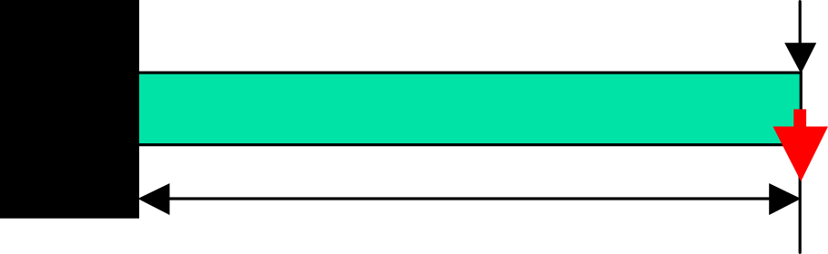 Figure 9.1.3 Verification Model
Table 9.1.8 exI: Verification Results (Maximum-Deflection History)
| Case Name | 0.1 | 0.2 | 0.3 | 0.4 | 0.5 | 0.6 | 0.7 | 0.8 | 0.9 | 1.0 | Linear Solution |
|---|---|---|---|---|---|---|---|---|---|---|---|
| I231 | - | - | - | - | - | - | - | - | - | - | - |
| I232 | - | - | - | - | - | - | - | - | - | - | - |
| I241 | - | - | - | - | - | - | - | - | - | - | - |
| I242 | - | - | - | - | - | - | - | - | - | - | - |
| I341 | 0.039 | 0.077 | 0.116 | 0.154 | 0.193 | 0.232 | 0.270 | 0.309 | 0.348 | 0.386 | 0.386 |
| I342 | 0.099 | 0.200 | 0.300 | 0.400 | 0.499 | 0.599 | 0.698 | 0.797 | 0.896 | 0.995 | 0.999 |
| I351 | 0.035 | 0.070 | 0.105 | 0.141 | 0.176 | 0.211 | 0.246 | 0.281 | 0.316 | 0.351 | 0.351 |
| I352 | 0.099 | 0.198 | 0.298 | 0.397 | 0.496 | 0.595 | 0.693 | 0.792 | 0.890 | 0.987 | 0.992 |
| I361 | 0.070 | 0.139 | 0.209 | 0.278 | 0.348 | 0.417 | 0.487 | 0.556 | 0.625 | 0.694 | 0.984 |
| I362 | 0.099 | 0.197 | 0.298 | 0.397 | 0.496 | 0.595 | 0.694 | 0.793 | 0.891 | 0.988 | 0.993 |
(2-2) exnl2: Elastoplastic Deformation Analysis
This verification problem is based on NAFEMS Test NL1 from the National Agency for Finite Element Methods and Standards (U.K.), and evaluates elastoplastic deformation with geometric nonlinearity and multiple hardening laws. Figure 9.1.4 shows the analysis model.
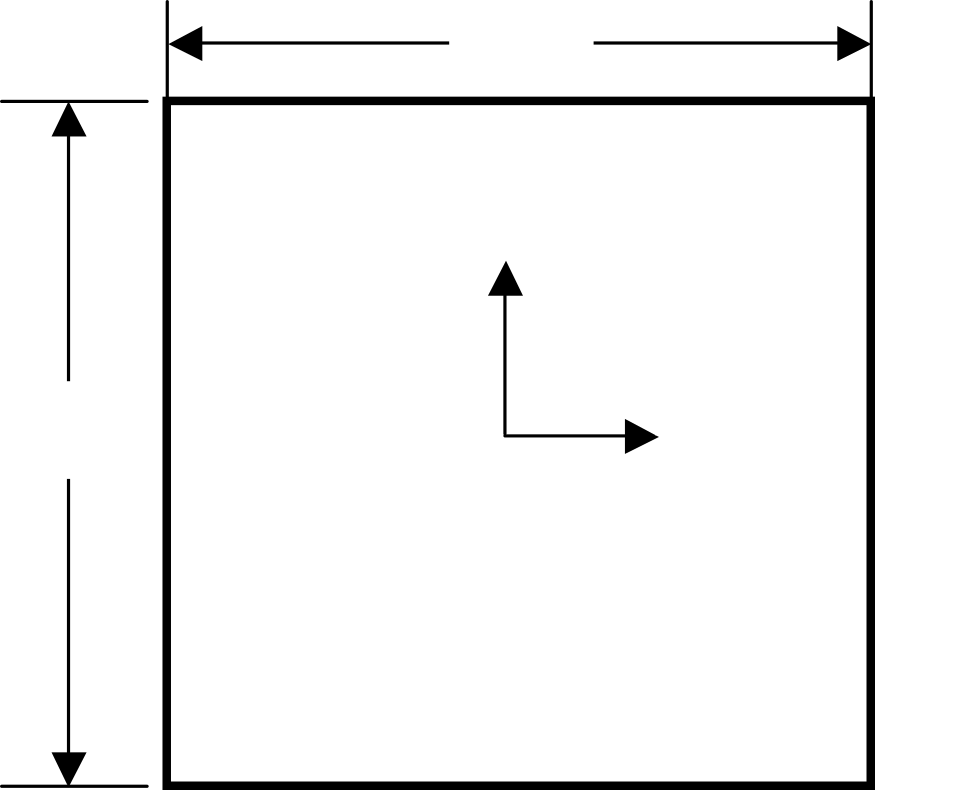
Figure 9.1.4 Elastoplastic Deformation Analysis Model
(1) Verification Conditions
| Item | Value |
|---|---|
| Material | Mises elastoplastic material |
| Young's modulus | \(E = 250\ \mathrm{GPa}\) |
| Poisson's ratio | \(\nu=0.25\) |
| Initial yield stress | \(5\ \mathrm{MPa}\) |
| Initial yield strain | \(0.25\times10^{-4}\) |
| Isotropic hardening coefficient | \(H_i = 0\) or \(62.5\ \mathrm{GPa}\) |
(2) Boundary Conditions
| Item | Boundary Condition | Value |
|---|---|---|
| Step 1 | Prescribed displacement at nodes 2 and 3 | \(u_x = 0.2500031251 * 10^{-4}\) |
| Step 2 | Prescribed displacement at nodes 2 and 3 | \(u_x = 0.25000937518 * 10^{-4}\) |
| Step 3 | Prescribed displacement at nodes 3 and 4 | \(u_y = 0.2500031251 * 10^{-4}\) |
| Step 4 | Prescribed displacement at nodes 3 and 4 | \(u_y = 0.25000937518 * 10^{-4}\) |
| Step 5 | Prescribed displacement at nodes 2 and 3 | \(u_x = -0.25000937518 * 10^{-4}\) |
| Step 6 | Prescribed displacement at nodes 2 and 3 | \(u_x = -0.2500031251 * 10^{-4}\) |
| Step 7 | Prescribed displacement at nodes 3 and 4 | \(u_y = -0.25000937518 * 10^{-4}\) |
| Step 8 | Prescribed displacement at nodes 3 and 4 | \(u_y = -0.2500031251 * 10^{-4}\) |
All nodes not listed here are fully constrained. The theoretical solution for this problem is as follows.
| Strain (\(\times10^{-4}\)) [\(\varepsilon_x\), \(\varepsilon_y\), \(\varepsilon_z\)] | Equivalent stress (MPa) [\(H_i=0\ H_k=0\); \(H_i=62.5\ H_k=0\)] |
|---|---|
| 0.25, 0, 0 | 5.0; 5.0 |
| 0.50, 0, 0 | 5.0; 5.862 |
| 0.50, 0.25, 0 | 5.0; 5.482 |
| 0.50, 0.50, 0 | 5.0; 6.362 |
| 0.25, 0.50, 0 | 5.0; 6.640 |
| 0, 0.50, 0 | 5.0; 7.322 |
| 0, 0.25, 0 | 3.917; 4.230 |
| 0, 0, 0 | 5.0; 5.673 |
The calculation results are as follows.
| Strain (\(\times10^{-4}\)) [\(\varepsilon_x\), \(\varepsilon_y\), \(\varepsilon_z\)] | Equivalent stress (MPa) [\(H_i=0\ H_k=0\); \(H_i=62.5\ H_k=0\)] |
|---|---|
| \(\varepsilon_{x}\) | \(\varepsilon_{y}\) |
| 0.25, 0, 0 | 5.0 (0.0%); 5.0 (0.0%) |
| 0.50, 0, 0 | 5.0 (0.0%); 5.862 (0.0%) |
| 0.50, 0.25, 0 | 5.0 (0.0%); 5.482 (0.0%) |
| 0.50, 0.50, 0 | 5.0 (0.0%); 6.362 (-0.05%) |
| 0.25, 0.50, 0 | 5.0 (0.0%); 6.640 (-0.21%) |
| 0, 0.50, 0 | 5.0 (0.0%); 7.322 (-0.34%) |
| 0, 0.25, 0 | 3.824 (-2.4%); 4.230 (-2.70%) |
| 0, 0, 0 | 5.0 (0.0%); 5.673 (5.673 (-2.50%) |
Contact Analysis (1)
This verification problem is based on contact patch test CGS-4 from the National Agency for Finite Element Methods and Standards (U.K.), and tests the finite-sliding contact capability with friction. Figure 9.1.5 shows the analysis model.
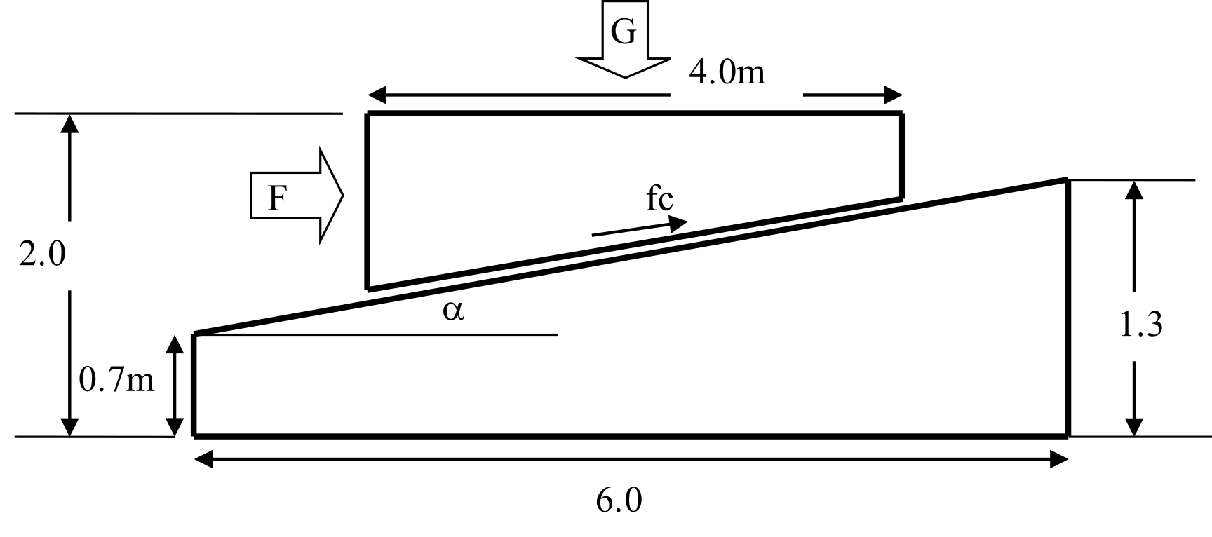
Figure 9.1.5 Contact Analysis Model
The equilibrium condition for this problem is as follows.
In the sticking-friction stage, the friction force is
whereas in the sliding-friction stage, it is
This gives the relation above.
The calculated results are compared with the analytical solution below.
| \(\mu\) | \(F/G\) Analytical Solution | \(F/G\) Calculated Result |
|---|---|---|
| 0.0 | 0.1 | 0.1 |
| 0.1 | 0.202 | 0.202 |
| 0.2 | 0.306 | 0.306 |
| 0.3 | 0.412 | 0.412 |
Contact Analysis (2): Hertz Contact Problem
This verification analyzes the Hertz contact problem between an infinitely long cylinder and an infinite plane. The cylinder radius is \(R = 8\ \mathrm{mm}\), and the Young's modulus \(E\) and Poisson's ratio \(\mu\) of the deformable body are \(1100\ \mathrm{MPa}\) and \(0.0\), respectively. The contact area is assumed to be sufficiently small relative to the cylinder radius. Accounting for symmetry, the analysis uses a quarter-cylinder model.
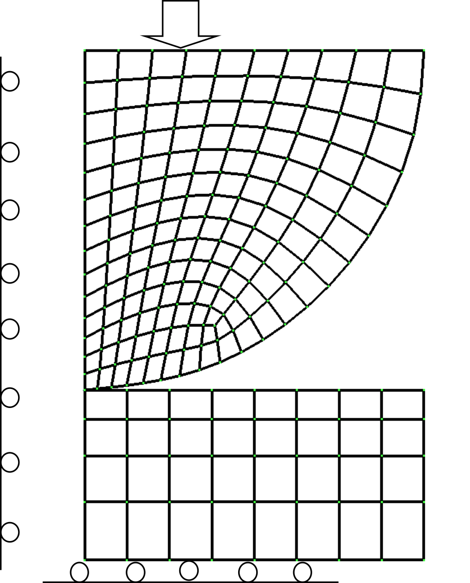 Figure 9.1.6 Analysis Model for the Hertz Contact Problem
(1) Verification Results for the Contact Radius
The theoretical equation for calculating the contact radius is as follows.
where
This gives the expression above. For the present calculation, when the pressure is \(F=100\), the contact radius is \(a=1.36\).
Figure 9.1.7 shows the equivalent nodal forces at the contact points. The contact radius is obtained by extrapolating this nodal-force distribution.
Figure 9.1.7 Equivalent Nodal-Force Distribution at the Contact Points
(2) Verification Results for the Maximum Shear Stress
In the theoretical solution, at the contact position
the maximum shear stress is
This is the theoretical maximum shear stress. For the present calculation conditions,
This is the theoretical value under the present conditions. The calculation, however, gives
This is the calculated result.
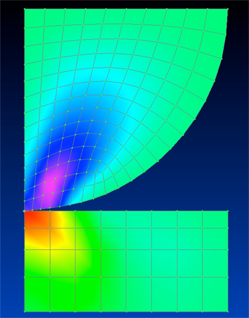 Figure 9.1.8 Shear-Stress Distribution (Maximum Value = 15.6)
(3) Modal Analysis
The verification models for cases exJ and exK are identical to those for cases exA through exG. Figure 9.1.9 shows a schematic of the verification model. Modal analysis is performed on this model. The first through third natural frequencies are calculated. Case exJ uses an iterative solver, whereas case exK uses a direct solver. The verification results are shown in Tables 9.1.9 through 9.1.12.
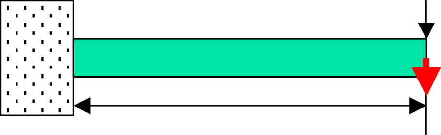 Figure 9.1.9 Verification Model
The natural frequencies of the cantilever beam are given by the following equations.
First natural frequency
Second natural frequency
Third natural frequency
The properties of the verification model are
| Item | Value |
|---|---|
| \(I\) | \(1.0/12.0\ \mathrm{mm}^4\) |
| \(E\) | \(4000.0\ \mathrm{kgf/mm^2}\) |
| \(l\) | \(10.0\ \mathrm{mm}\) |
| \(\omega\) | \(7.85 \times 10^{-6}\ \mathrm{kgf/mm^3}\) |
| \(g\) | \(9800.0\ \mathrm{mm/s^2}\) |
Thus, the first three natural frequencies are as follows.
| Mode Number | Value |
|---|---|
| \(n_1\) | 3.609e3 |
| \(n_2\) | 2.262e4 |
| \(n_3\) | 6.335e4 |
Table 9.1.9 exJ: Iterative-Solver Verification Results (First Natural Frequency)
| Case Name | Number of Elements | Predicted Value: n1=3.609e3 | Remarks | |
|---|---|---|---|---|
| NASTRAN | FrontISTR | |||
| J231 | 40 | 5.861e3 | 5.861e3 | 33 nodes / plane-stress problem |
| J232 | 40 | 3.596e3 | 3.593e3 | 105 nodes / plane-stress problem |
| J241 | 20 | 3.586e3 | 4.245e3 | 33 nodes / plane-stress problem |
| J242 | 20 | 3.590e3 | 3.587e3 | 85 nodes / plane-stress problem |
| J341 | 240 | 5.442e3 | 5.429e3 | 99 nodes |
| J342 | 240 | 3.621e3 | 3.595e3 | 525 nodes |
| J351 | 80 | 3.695e3 | 4.298e3 | 99 nodes |
| J352 | 80 | 3.610e3 | 3.609e3 | 381 nodes |
| J361 | 40 | 3.679e3 | 3.619e3 | 99 nodes |
| J362 | 40 | 3.611e3 | 3.606e3 | 220 nodes |
Table 9.1.10 exJ: Iterative-Solver Verification Results (Second Natural Frequency)
| Case Name | Number of Elements | Predicted Value: n2=2.262e4 | Remarks | |
|---|---|---|---|---|
| NASTRAN | FrontISTR | |||
| J231 | 40 | 3.350e4 | 3.351e4 | 33 nodes / plane-stress problem |
| J232 | 40 | 2.163e4 | 2.156e4 | 105 nodes / plane-stress problem |
| J241 | 20 | 2.149e4 | 2.516e4 | 33 nodes / plane-stress problem |
| J242 | 20 | 2.149e4 | 2.143e4 | 85 nodes / plane-stress problem |
| J341 | 240 | 3.145e4 | 3.138e4 | 99 nodes |
| J342 | 240 | 2.171e4 | 2.155e4 | 525 nodes |
| J351 | 80 | 2.208e4 | 2.546e4 | 99 nodes |
| J352 | 80 | 2.156e4 | 2.149e4 | 381 nodes |
| J361 | 40 | 2.202e4 | 2.168e4 | 99 nodes |
| J362 | 40 | 2.154e4 | 2.144e4 | 220 nodes |
Note: In three-dimensional models, the first two modes are degenerate; therefore, the third computed natural frequency is reported as the second natural frequency in the table.
Table 9.1.11 exK: Direct-Solver Verification Results (First Natural Frequency)
| Case Name | Number of Elements | Predicted Value: n1=3.609e3 | Remarks | |
|---|---|---|---|---|
| NASTRAN | FrontISTR | |||
| J231 | 40 | 5.861e3 | 5.861e3 | 33 nodes / plane-stress problem |
| J232 | 40 | 3.596e3 | 3.593e3 | 105 nodes / plane-stress problem |
| J241 | 20 | 3.586e3 | 4.245e3 | 33 nodes / plane-stress problem |
| J242 | 20 | 3.590e3 | 3.587e3 | 85 nodes / plane-stress problem |
| J341 | 240 | 5.442e3 | 5.429e3 | 99 nodes |
| J342 | 240 | 3.621e3 | 3.595e3 | 525 nodes |
| J351 | 80 | 3.695e3 | 4.298e3 | 99 nodes |
| J352 | 80 | 3.610e3 | 3.609e3 | 381 nodes |
| J361 | 40 | 3.679e3 | 3.619e3 | 99 nodes |
| J362 | 40 | 3.611e3 | 3.606e3 | 220 nodes |
| J731 | 40 | - | 3.606e3 | 220 nodes |
| J741 | 20 | - | 3.594e3 | 220 nodes |
Table 9.1.12 exK: Direct-Solver Verification Results (Second Natural Frequency)
| Case Name | Number of Elements | Predicted Value: n2=2.262e4 | Remarks | |
|---|---|---|---|---|
| NASTRAN | FrontISTR | |||
| J231 | 40 | 3.350e4 | 3.351e4 | 33 nodes / plane-stress problem |
| J232 | 40 | 2.163e4 | 2.156e4 | 105 nodes / plane-stress problem |
| J241 | 20 | 2.149e4 | 2.516e4 | 33 nodes / plane-stress problem |
| J242 | 20 | 2.149e4 | 2.143e4 | 85 nodes / plane-stress problem |
| J341 | 240 | 3.145e4 | 3.138e4 | 99 nodes |
| J342 | 240 | 2.171e4 | 2.155e4 | 525 nodes |
| J351 | 80 | 2.208e4 | 2.546e4 | 99 nodes |
| J352 | 80 | 2.156e4 | 2.149e4 | 381 nodes |
| J361 | 40 | 2.202e4 | 2.168e4 | 99 nodes |
| J362 | 40 | 2.154e4 | 2.144e4 | 220 nodes |
| J731 | 40 | - | 2.156e4 | 220 nodes |
| J741 | 20 | - | 2.153e4 | 220 nodes |
Note: In three-dimensional models, the first two modes are degenerate; therefore, the third computed natural frequency is reported as the second natural frequency in the table.
(4) Heat Conduction Analysis
The common conditions for steady-state heat conduction analysis are shown in Figure 9.1.10. The individual conditions for verification cases exM through exT are shown in Figure 9.1.11. The same mesh as for exA is used.
Tables 9.1.13 through 9.1.20 show the temperature-distribution results for each case.
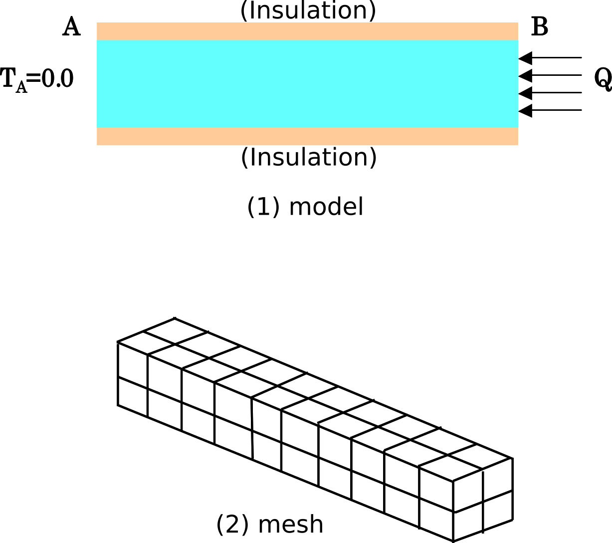
| Distance between A and B | \(L = 10.0\ \mathrm{m}\) |
| Cross-sectional area | \(A = 1.0\ \mathrm{m^2}\) |
Temperature Dependence of Thermal Conductivity
| Thermal Conductivity \(\lambda\) (W/(m·K)) | Temperature (°C) |
|---|---|
| 50.0 | 0.0 |
| 35.0 | 500.0 |
| 20.0 | 1000.0 |
Figure 9.1.10 Verification Conditions for Steady-State Heat Conduction Analysis
| exM: Linear material | |
| exN: Prescribed-temperature problem |  |
| exO: Concentrated heat-flux problem | 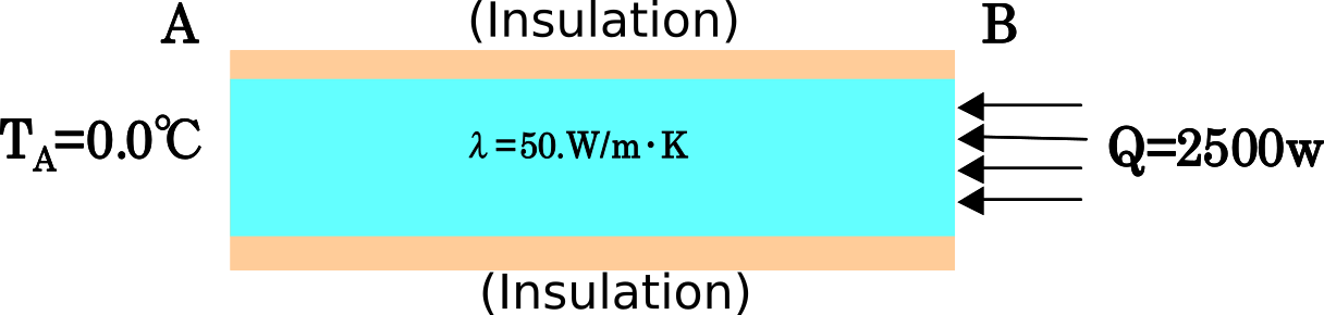 |
| exP: Distributed heat-flux problem |  |
| exQ: Convective heat-transfer problem | 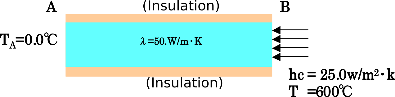 |
| exR: Radiative heat-transfer problem | 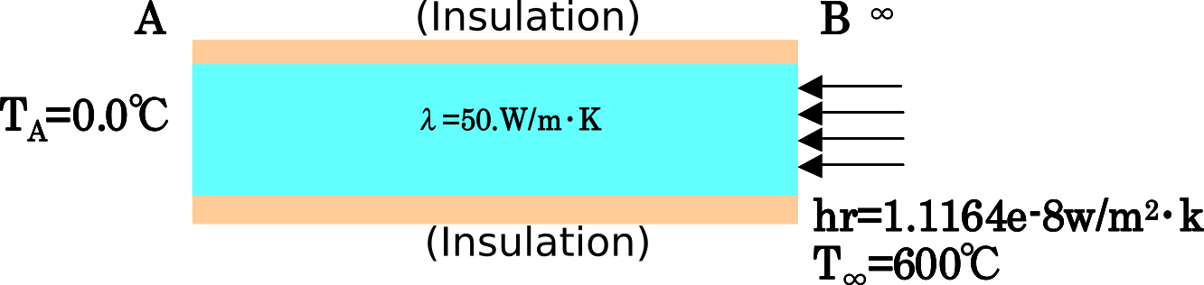 |
| exS: Volumetric heat-generation problem | 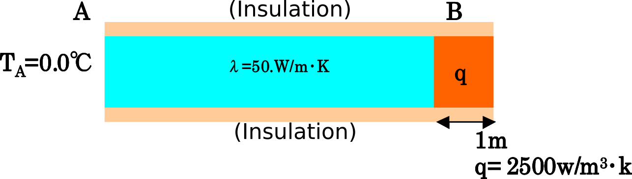 |
| exT: Internal-gap problem | 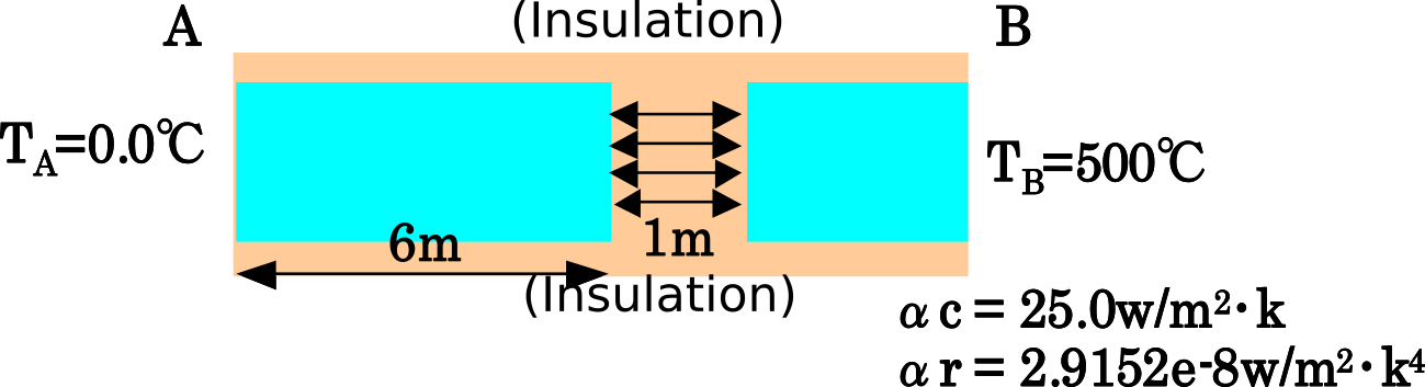 |
Figure 9.1.11 Analysis Conditions for Each Verification Case
Table 9.1.13 exM: Verification Results for Steady-State Calculation with a Linear Material
| Case Name | Element Type | Elements/Nodes | Distance from End A (m) | |||||
|---|---|---|---|---|---|---|---|---|
| End A | 2.0 | 4.0 | 6.0 | 8,0 | End B | |||
| M361A | 361 | 40/33 | 0.0 | 100.0 | 200.0 | 300.0 | 400.0 | 500.0 |
| M361B | 361 | 40/105 | 0.0 | 100.0 | 200.0 | 300.0 | 400.0 | 500.0 |
| M361C | 361 | 20/33 | 0.0 | 100.0 | 200.0 | 300.0 | 400.0 | 500.0 |
| M361D | 361 | 20/85 | 0.0 | 100.0 | 200.0 | 300.0 | 400.0 | 500.0 |
| M361E | 361 | 240/99 | 0.0 | 100.0 | 200.0 | 300.0 | 400.0 | 500.0 |
| M361F | 361 | 24/525 | 0.0 | 100.0 | 200.0 | 300.0 | 400.0 | 500.0 |
| M361G | 361 | 80/99 | 0.0 | 100.0 | 200.0 | 300.0 | 400.0 | 500.0 |
Table 9.1.14 exN: Verification Results for the Prescribed-Temperature Problem
| Case Name | Element Type | Elements/Nodes | Distance from End A (m) | |||||
|---|---|---|---|---|---|---|---|---|
| End A | 2.0 | 4.0 | 6.0 | 8,0 | End B | |||
| Commercial Software | 361 | 40/99 | 0.0 | 87.3 | 179.7 | 278.2 | 384.3 | 500.0 |
| N231 | 231 | 40/33 | 0.0 | 87.2 | 179.5 | 278.0 | 384.1 | 500.0 |
| N232 | 232 | 40/105 | 0.0 | 86.0 | 178.3 | 276.8 | 382.9 | 500.0 |
| N241 | 241 | 20/33 | 0.0 | 87.3 | 179.7 | 278.2 | 384.3 | 500.0 |
| N242 | 242 | 20/85 | 0.0 | 87.3 | 179.7 | 278.2 | 384.3 | 500.0 |
| N341 | 341 | 240/99 | 0.0 | 87.3 | 179.7 | 278.2 | 384.3 | 500.0 |
| N342 | 342 | 24/525 | 0.0 | 87.9 | 179.9 | 278.0 | 383.6 | 500.0 |
| N351 | 351 | 80/99 | 0.0 | 87.3 | 179.7 | 278.2 | 384.3 | 500.0 |
| N352 | 352 | 80/381 | 0.0 | 87.3 | 179.7 | 278.2 | 384.3 | 500.0 |
| N361 | 361 | 40/99 | 0.0 | 87.3 | 179.7 | 278.2 | 384.3 | 500.0 |
| N362 | 362 | 40/330 | 0.0 | 87.3 | 179.7 | 278.2 | 384.3 | 500.0 |
| N731 | 731 | 40/33 | 0.0 | 87.3 | 179.7 | 278.2 | 384.3 | 500.0 |
| N741 | 741 | 20/33 | 0.0 | 87.3 | 179.7 | 278.2 | 384.3 | 500.0 |
Table 9.1.15 exO: Verification Results for the Concentrated-Heat-Flux Problem
| Case Name | Element Type | Elements/Nodes | Distance from End A (m) | |||||
|---|---|---|---|---|---|---|---|---|
| End A | 2.0 | 4.0 | 6.0 | 8,0 | End B | |||
| Commercial Software | 361 | 40/99 | 0.0 | 103.2 | 213.7 | 333.3 | 464.8 | 612.6 |
| O231 | 231 | 40/33 | 0.0 | 103.2 | 213.7 | 333.3 | 464.8 | 612.6 |
| O232 | 232 | 40/105 | 0.0 | 103.2 | 213.7 | 333.3 | 464.8 | 612.6 |
| O241 | 241 | 20/33 | 0.0 | 103.2 | 213.7 | 333.3 | 464.8 | 612.6 |
| O242 | 242 | 20/85 | 0.0 | 103.2 | 213.7 | 333.4 | 465.2 | 618.0 |
| O341 | 341 | 240/99 | - | - | - | - | - | - |
| O342 | 342 | 24/525 | 0.0 | 104.4 | 214.9 | 334.7 | 466.3 | 614.6 |
| O351 | 351 | 80/99 | - | - | - | - | - | - |
| O352 | 352 | 80/381 | 0.0 | 103.2 | 213.7 | 333.3 | 465.0 | 624.2 |
| O361 | 361 | 40/99 | 0.0 | 103.2 | 213.7 | 333.3 | 464.8 | 612.6 |
| O362 | 362 | 40/330 | 0.0 | 103.2 | 213.7 | 333.4 | 465.5 | 623.5 |
| O731 | 731 | 40/33 | 0.0 | 103.2 | 213.7 | 333.3 | 464.8 | 612.5 |
| O741 | 741 | 20/33 | 0.0 | 103.2 | 213.7 | 333.3 | 464.8 | 612.6 |
Table 9.1.16 exP: Verification Results for the Distributed-Heat-Flux Problem
| Case Name | Element Type | Elements/Nodes | Distance from End A (m) | |||||
|---|---|---|---|---|---|---|---|---|
| End A | 2.0 | 4.0 | 6.0 | 8,0 | End B | |||
| Commercial Software | 361 | 40/99 | 0.0 | 103.2 | 213.7 | 333.3 | 464.8 | 612.6 |
| P231 | 231 | 40/33 | 0.0 | 103.2 | 213.7 | 333.3 | 464.8 | 612.6 |
| P232 | 232 | 40/105 | 0.0 | 103.2 | 213.7 | 333.3 | 464.8 | 612.6 |
| P241 | 241 | 20/33 | 0.0 | 103.2 | 213.7 | 333.3 | 464.8 | 612.6 |
| P242 | 242 | 20/85 | 0.0 | 103.2 | 213.7 | 333.3 | 464.8 | 612.6 |
| P341 | 341 | 240/99 | - | - | - | - | - | - |
| P342 | 342 | 24/525 | 0.0 | 103.2 | 213.7 | 333.3 | 464.8 | 612.6 |
| P351 | 351 | 80/99 | - | - | - | - | - | - |
| P352 | 352 | 80/381 | 0.0 | 103.2 | 213.7 | 333.3 | 464.8 | 612.6 |
| P361 | 361 | 40/99 | 0.0 | 103.2 | 213.7 | 333.3 | 464.8 | 612.6 |
| P362 | 362 | 40/330 | 0.0 | 103.2 | 213.7 | 333.4 | 465.5 | 612.6 |
| P731 | 731 | 40/33 | 0.0 | 103.2 | 213.7 | 333.3 | 464.8 | 612.5 |
| P741 | 741 | 20/33 | 0.0 | 103.2 | 213.7 | 333.3 | 464.8 | 612.6 |
Table 9.1.17 exQ: Verification Results for the Convective-Heat-Transfer Problem
| Case Name | Element Type | Elements/Nodes | Distance from End A (m) | |||||
|---|---|---|---|---|---|---|---|---|
| End A | 2.0 | 4.0 | 6.0 | 8,0 | End B | |||
| Commercial Software | 361 | 40/99 | 0.0 | 89.2 | 183.8 | 284.8 | 393.9 | 513.2 |
| Q231 | 231 | 40/33 | 0.0 | 89.2 | 183.8 | 284.8 | 393.9 | 513.2 |
| Q232 | 232 | 40/105 | 0.0 | 89.2 | 183.8 | 284.8 | 393.9 | 513.2 |
| Q241 | 241 | 20/33 | 0.0 | 89.2 | 183.8 | 284.8 | 393.9 | 513.2 |
| Q242 | 242 | 20/85 | 0.0 | 89.2 | 183.8 | 284.8 | 393.9 | 513.2 |
| Q341 | 341 | 240/99 | - | - | - | - | - | - |
| Q342 | 342 | 24/525 | 0.0 | 89.2 | 183.8 | 284.8 | 393.9 | 513.2 |
| Q351 | 351 | 80/99 | - | - | - | - | - | - |
| Q352 | 352 | 80/381 | 0.0 | 89.2 | 183.8 | 284.8 | 393.9 | 513.2 |
| Q361 | 361 | 40/99 | 0.0 | 89.2 | 183.8 | 284.8 | 393.9 | 513.2 |
| Q362 | 362 | 40/330 | 0.0 | 89.2 | 183.8 | 284.8 | 393.9 | 513.2 |
| Q731 | 731 | 40/33 | 0.0 | 89.2 | 183.8 | 284.8 | 393.9 | 513.2 |
| Q741 | 741 | 20/33 | 0.0 | 89.2 | 183.8 | 284.8 | 393.9 | 513.2 |
Table 9.1.18 exR: Verification Results for the Radiative-Heat-Transfer Problem
| Case Name | Element Type | Elements/Nodes | Distance from End A (m) | |||||
|---|---|---|---|---|---|---|---|---|
| End A | 2.0 | 4.0 | 6.0 | 8,0 | End B | |||
| Commercial Software | 361 | 40/99 | 0.0 | 89.5 | 184.4 | 285.8 | 395.3 | 515.2 |
| R231 | 231 | 40/33 | 0.0 | 89.5 | 184.4 | 285.8 | 395.3 | 515.2 |
| R232 | 232 | 40/105 | 0.0 | 89.5 | 184.4 | 285.8 | 395.3 | 515.2 |
| R241 | 241 | 20/33 | 0.0 | 89.5 | 184.4 | 285.8 | 395.3 | 515.2 |
| R242 | 242 | 20/85 | 0.0 | 89.5 | 184.4 | 285.8 | 395.3 | 515.2 |
| R341 | 341 | 240/99 | - | - | - | - | - | - |
| R342 | 342 | 24/525 | 0.0 | 89.5 | 184.4 | 285.8 | 395.3 | 515.2 |
| R351 | 351 | 80/99 | - | - | - | - | - | - |
| R352 | 352 | 80/381 | 0.0 | 89.5 | 184.4 | 285.8 | 395.3 | 515.2 |
| R361 | 361 | 40/99 | 0.0 | 89.5 | 184.4 | 285.8 | 395.3 | 515.2 |
| R362 | 362 | 40/330 | 0.0 | 89.5 | 184.4 | 285.8 | 395.3 | 515.2 |
| R731 | 731 | 40/33 | 0.0 | 89.5 | 184.4 | 285.8 | 395.3 | 515.2 |
| R741 | 741 | 20/33 | 0.0 | 89.5 | 184.4 | 285.8 | 395.3 | 515.2 |
Table 9.1.19 exS: Verification Results for the Volumetric-Heat-Generation Problem
| Case Name | Element Type | Elements/Nodes | Distance from End A (m) | |||||
|---|---|---|---|---|---|---|---|---|
| End A | 2.0 | 4.0 | 6.0 | 8,0 | End B | |||
| Commercial Software | 361 | 40/99 | 0.0 | 103.2 | 213.7 | 333.3 | 464.8 | 612.6 |
| S231 | 231 | 40/33 | 0.0 | 103.2 | 213.7 | 333.3 | 464.8 | 612.6 |
| S232 | 232 | 40/105 | 0.0 | 103.2 | 213.7 | 333.3 | 464.8 | 612.6 |
| S241 | 241 | 20/33 | 0.0 | 103.2 | 213.7 | 333.3 | 464.8 | 612.6 |
| S242 | 242 | 20/85 | 0.0 | 103.2 | 213.7 | 333.3 | 464.8 | 612.6 |
| S341 | 341 | 240/99 | - | - | - | - | - | - |
| S342 | 342 | 24/525 | 0.0 | 103.2 | 213.7 | 333.3 | 464.8 | 612.6 |
| S351 | 351 | 80/99 | - | - | - | - | - | - |
| S352 | 352 | 80/381 | 0.0 | 103.2 | 213.7 | 333.3 | 464.8 | 612.6 |
| S361 | 361 | 40/99 | 0.0 | 103.2 | 213.7 | 333.3 | 464.8 | 612.6 |
| S362 | 362 | 40/330 | 0.0 | 103.2 | 213.7 | 333.3 | 464.8 | 612.6 |
| S731 | 731 | 40/33 | 0.0 | 103.2 | 213.7 | 333.3 | 464.8 | 612.6 |
| S741 | 741 | 20/33 | 0.0 | 103.2 | 213.7 | 333.3 | 464.8 | 612.6 |
Table 9.1.20 exT: Verification Results for the Internal-Gap Problem
| Case Name | Element Type | Elements/Nodes | Distance from End A (m) | |||||
|---|---|---|---|---|---|---|---|---|
| End A | 2.0 | 4.0 | 6.0 | 8,0 | End B | |||
| Commercial Software | 361 | 40/99 | 0.0 | 88.6 | 182.4 | 282.6 | 387.7 | 500.0 |
| S231 | 231 | 40/33 | 0.0 | 88.6 | 182.4 | 282.6 | 387.7 | 500.0 |
| S232 | 232 | 40/105 | 0.0 | 88.6 | 182.4 | 282.6 | 387.7 | 500.0 |
| S241 | 241 | 20/33 | 0.0 | 88.6 | 182.4 | 282.6 | 387.7 | 500.0 |
| S242 | 242 | 20/85 | 0.0 | 88.6 | 182.4 | 282.6 | 387.7 | 500.0 |
| S341 | 341 | 240/99 | - | - | - | - | - | - |
| S342 | 342 | 24/525 | 0.0 | 88.6 | 182.4 | 282.6 | 387.7 | 500.0 |
| S351 | 351 | 80/99 | - | - | - | - | - | - |
| S352 | 352 | 80/381 | 0.0 | 88.6 | 182.4 | 282.6 | 387.7 | 500.0 |
| S361 | 361 | 40/99 | 0.0 | 88.6 | 182.4 | 282.6 | 387.7 | 500.0 |
| S362 | 362 | 40/330 | 0.0 | 88.6 | 182.4 | 282.6 | 387.7 | 500.0 |
| S731 | 731 | 40/33 | 0.0 | 88.6 | 182.4 | 282.6 | 387.7 | 500.0 |
| S741 | 741 | 20/33 | 0.0 | 88.6 | 182.4 | 282.6 | 387.7 | 500.0 |
Linear Dynamic Analysis
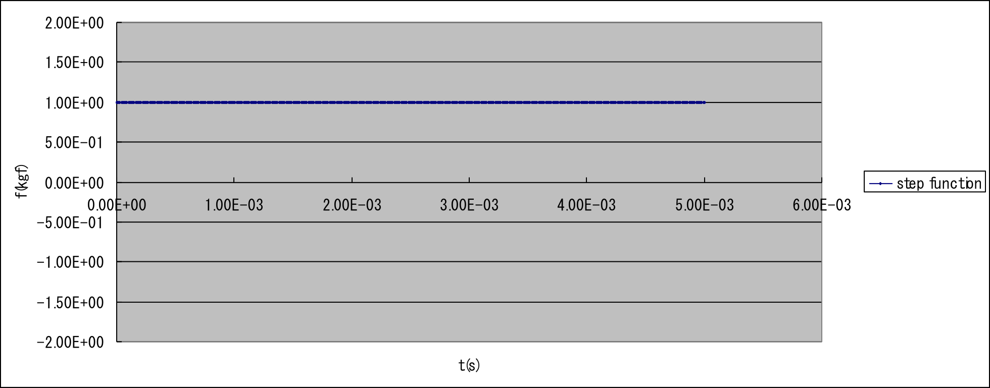
In exW, linear dynamic analysis is performed on the same cantilever beam as in Section (1). Figure 9.1.12 shows the verification conditions. The effect of the time increment is verified using the same mesh. Both implicit and explicit methods are used, with element types 361 and 342. The verification results are shown in Table 9.1.22 and Figures 9.1.13 through 9.1.15.
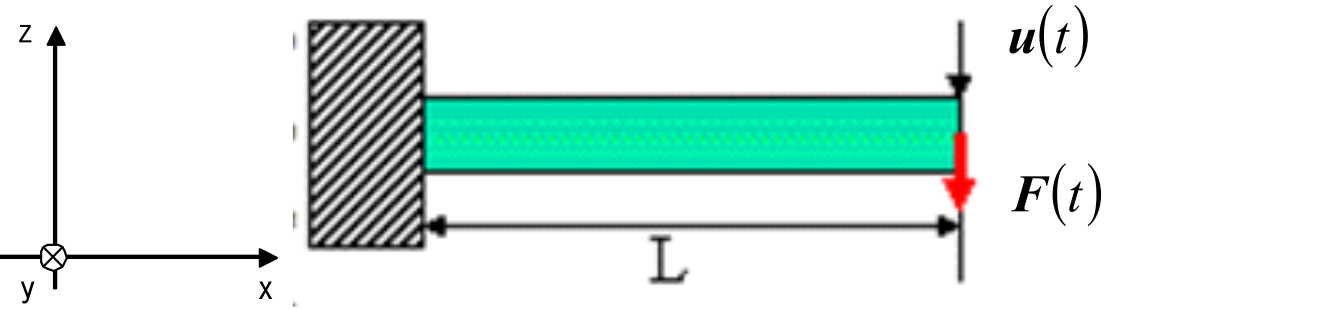 Analysis Model
 Time History of External Force F
The theoretical solution for displacement at the excitation point is as follows:
where
Figure 9.1.12 Verification Conditions for Linear Dynamic Analysis
Verification Conditions:
| Length | \(L\) | \(10.0\ \mathrm{mm}\) |
| Cross-sectional width | \(a\) | \(1.0\ \mathrm{mm}\) |
| Cross-sectional height | \(b\) | \(1.0\ \mathrm{mm}\) |
| Young's modulus | \(E\) | \(4000.0\ \mathrm{kgf/mm^2}\) |
| Poisson's ratio | \(\nu\) | \(0.3\) |
| Density | \(\rho\) | \(1.0 \times 10^{-9}\ \mathrm{kgf}\;\mathrm{s}^2/\mathrm{mm}^4\) |
| Gravitational acceleration | \(g\) | \(9800.0\ \mathrm{mm/s^2}\) |
| External force | \(F_0\) | \(1.0\ \mathrm{kgf}\) |
| Element | First-order hexahedral element |
| Second-order tetrahedral element | |
| Solution Method | Implicit method |
| Newmark-\(\beta\) method parameter \(\gamma\) | 1/2 |
| Newmark-\(\beta\) method parameter \(\beta\) | 1/4 |
| Explicit method | |
| Damping | None |
Table 9.1.21 Verification Conditions for Linear Dynamic Analysis (Continued)
| Case Name | Element Type | Number of Nodes | Number of Elements | Method | Time Increment \(\Delta t\) (s) |
|---|---|---|---|---|---|
| W361_c0_im_m2_t1 | 361 | 99 | 40 | Implicit method | 1.0E-06 |
| W361_c0_im_m2_t2 | 361 | 99 | 40 | Implicit method | 1.0E-05 |
| W361_c0_im_m2_t3 | 361 | 99 | 40 | Implicit method | 1.0E-04 |
| W361_c0_ex_m2_t1 | 361 | 99 | 40 | Implicit method | 1.0E-08 |
| W361_c0_ex_m2_t2 | 361 | 99 | 40 | Implicit method | 1.0E-07 |
| W361_c0_ex_m2_t3 | 361 | 99 | 40 | Implicit method | 1.0E-06 |
| W342_c0_im_m2_t1 | 342 | 525 | 240 | Explicit method | 1.0E-06 |
| W342_c0_im_m2_t2 | 342 | 525 | 240 | Explicit method | 1.0E-05 |
| W342_c0_im_m2_t3 | 342 | 525 | 240 | Explicit method | 1.0E-04 |
| W342_c0_ex_m2_t1 | 342 | 525 | 240 | Explicit method | 1.0E-08 |
| W342_c0_ex_m2_t2 | 342 | 525 | 240 | Explicit method | 5.0E-08 |
| W342_c0_ex_m2_t3 | 342 | 525 | 240 | Explicit method | 1.0E-07 |
Table 9.1.22 exW: Verification Results for Linear Dynamic Analysis of a Cantilever Beam
| Case Name | Element Type | Number of Nodes | Number of Elements | Method | z-Direction Displacement at Time \(t = 0.002\ \mathrm{s}\) (mm) | |
|---|---|---|---|---|---|---|
| W361_c0_im_m2_t1 | 361 | 99 | 40 | Implicit method | 1.9753 | 1.9302 |
| W361_c0_im_m2_t2 | 361 | 99 | 40 | Implicit method | 1.9753 | 1.8686 |
| W361_c0_im_m2_t3 | 361 | 99 | 40 | Implicit method | 1.9753 | 0.3794 |
| W361_c0_ex_m2_t1 | 361 | 99 | 40 | Implicit method | 1.9753 | 1.9302 |
| W361_c0_ex_m2_t2 | 361 | 99 | 40 | Implicit method | 1.9753 | 1.9247 |
| W361_c0_ex_m2_t3 | 361 | 99 | 40 | Implicit method | 1.9753 | Diverged |
| W342_c0_im_m2_t1 | 342 | 525 | 240 | Explicit method | 1.9753 | 1.9431 |
| W342_c0_im_m2_t2 | 342 | 525 | 240 | Explicit method | 1.9753 | 1.8719 |
| W342_c0_im_m2_t3 | 342 | 525 | 240 | Explicit method | 1.9753 | 0.3873 |
| W342_c0_ex_m2_t1 | 342 | 525 | 240 | Explicit method | 1.9753 | 1.9359 |
| W342_c0_ex_m2_t2 | 342 | 525 | 240 | Explicit method | 1.9753 | 1.9358 |
| W342_c0_ex_m2_t3 | 342 | 525 | 240 | Explicit method | 1.9753 | Diverged |
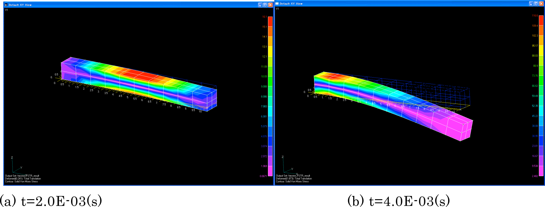 Figure 9.1.13 Deformed Shape and Equivalent Stress Distribution of the Cantilever Beam
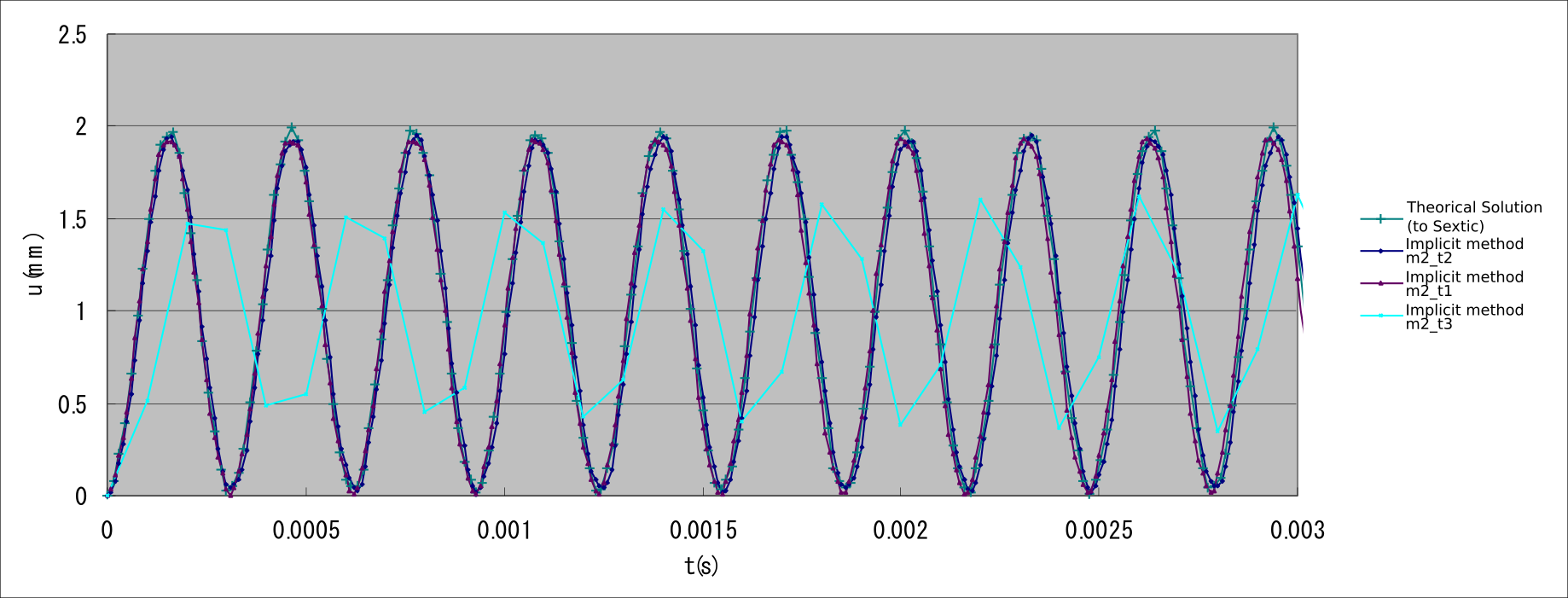 (a) Element Type 361: Implicit Method
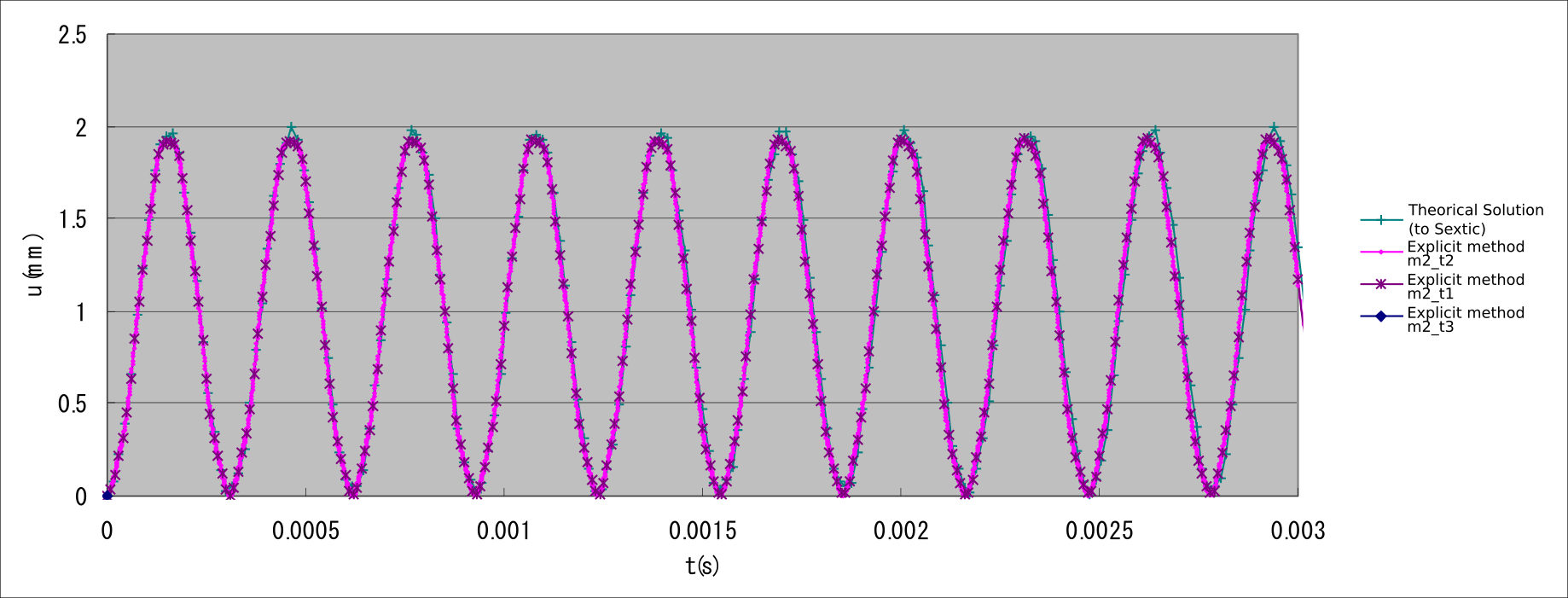 (b) Element Type 361: Explicit Method
Figure 9.1.14 Time History of Excitation-Point Displacement \(u_z\)
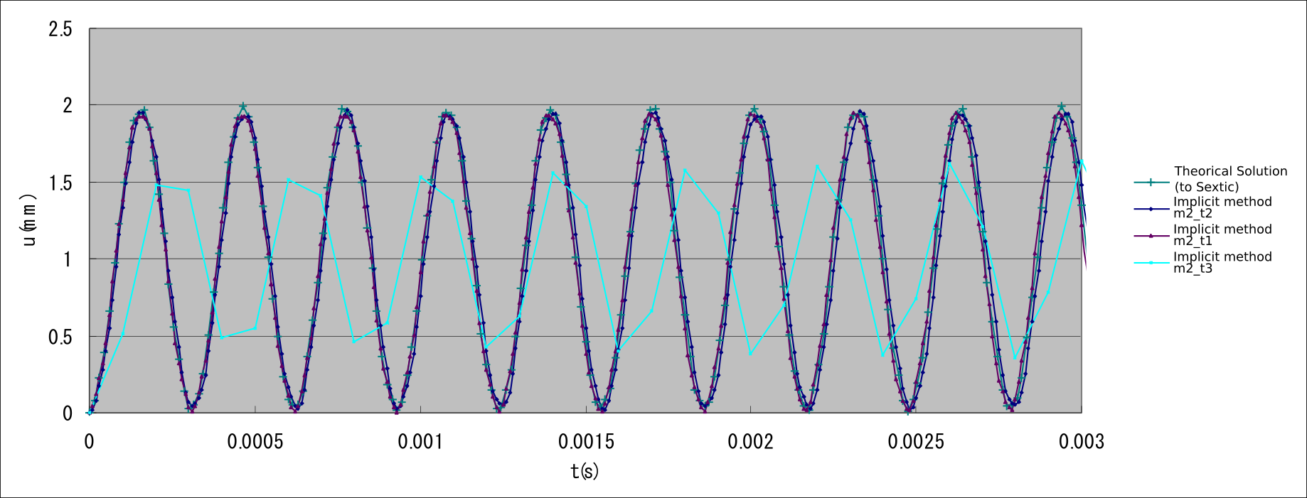 (a) Element Type 342: Implicit Method
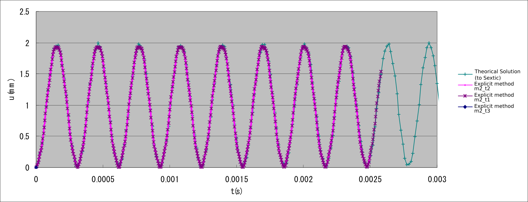 (b) Element Type 342: Explicit Method
Figure 9.1.15 Time History of Excitation-Point Displacement \(u_z\)
Frequency Response Analysis
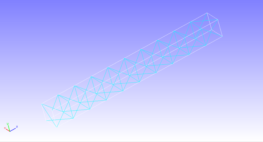
This verification performs frequency response analysis of a cantilever beam and compares the results with those from general-purpose commercial software. The analysis model and verification conditions are shown below.
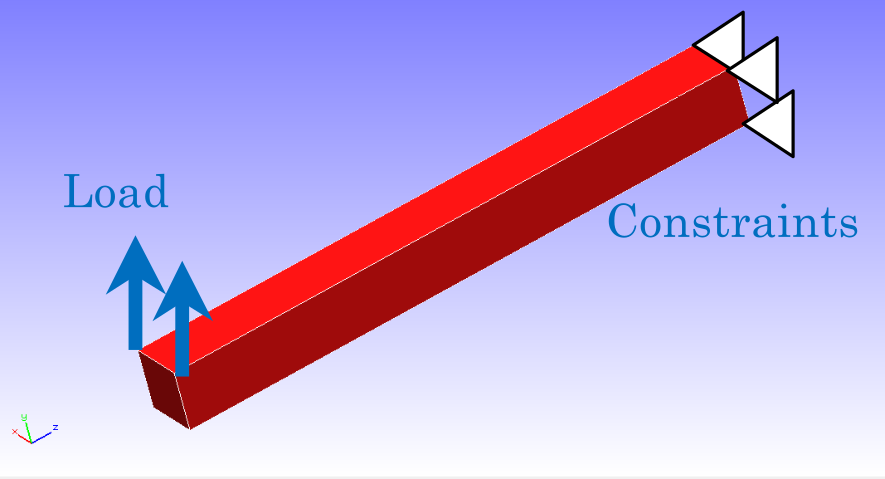
Analysis Conditions:
| Young's modulus | \(E\) | \(210000\ \mathrm{N/mm^2}\) |
| Poisson's ratio | \(\nu\) | \(0.3\) |
| Density | \(\rho\) | \(7.89 \times 10^{-9}\ \mathrm{t/mm^3}\) |
| Gravitational acceleration | \(g\) | \(9800.0\ \mathrm{mm/s^2}\) |
| Load | \(F_0\) | \(1.0\ \mathrm{N}\) |
| Rayleigh Damping Parameter | \(R_m\) | \(0.0\) |
| Rayleigh Damping Parameter | \(R_k\) | \(7.2E-07\) |
Figure 9.1.16 Analysis Model (First-Order Tetrahedral Elements: 126 Elements, 55 Nodes)
The first five natural frequencies obtained by modal analysis, together with the frequency response at the excitation point, are shown below.
| Mode | FrontISTR | Commercial Software |
|---|---|---|
| 1 | 14952 | 14952 |
| 2 | 15002 | 15003 |
| 3 | 84604 | 84539 |
| 4 | 84771 | 84697 |
| 5 | 127054 | 126852 |
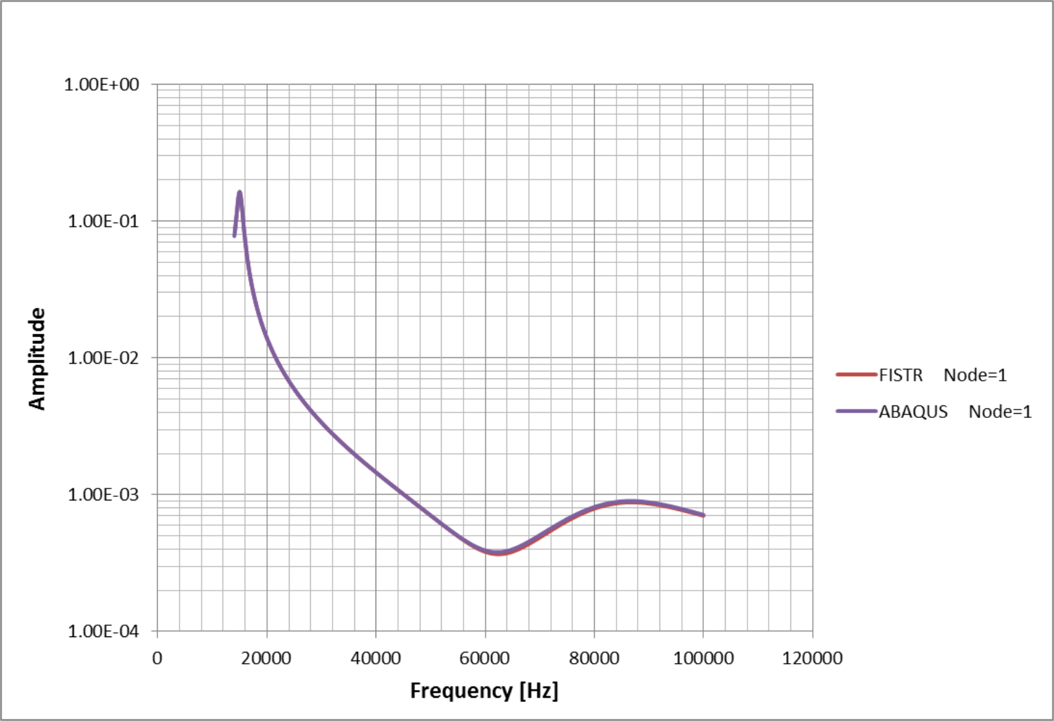 Figure 9.1.17 Frequency Dependence of Displacement Magnitude at the Excitation Point