Linear Elastic Static Analysis (Introduction)

This section presents the formulation of elastic static analysis based on infinitesimal deformation theory. Linear elasticity is assumed for the stress-strain relation. This chapter is intended as an introduction for understanding the overall structure of finite-element structural analysis and is organized as a self-contained chapter.

For the general theory of the principle of virtual work (current-configuration form, initial-configuration form, and reduction to infinitesimal deformation), see Principle of Virtual Work. For details of the linear-elastic constitutive law, see Linear Elasticity; for conventions of tensor and Voigt notation, see Tensor Notation and Mathematical Fundamentals; for the general formulation of finite deformation, see Fundamentals of Continuum Mechanics; and for solution methods for nonlinear problems, see Tangent Stiffness Matrix.

Basic Equations

Under the assumptions of infinitesimal deformation and linear elasticity, the boundary-value problem in solid mechanics consists of the equilibrium equation, mechanical boundary conditions, and geometric boundary conditions (essential boundary conditions) (see Figure 2.1.1):

\[\begin{equation} \nabla \cdot \boldsymbol{\sigma} + \overline{\boldsymbol{b}} = \boldsymbol{0} \quad \text{in} \ V \label{eq:2.1.1} \end{equation}\]

\[\begin{equation} \boldsymbol{\sigma} \cdot \boldsymbol{n} = \overline{\boldsymbol{t}} \quad \text{on} \ S_t \label{eq:2.1.2} \end{equation}\]

\[\begin{equation} \boldsymbol{u} = \overline{\boldsymbol{u}} \quad \text{on} \ S_u \label{eq:2.1.3} \end{equation}\]

Here, \(\boldsymbol{\sigma}\) is the Cauchy stress, \(\overline{\boldsymbol{b}}\) is the body force per unit volume, \(\overline{\boldsymbol{t}}\) is the prescribed surface traction, \(\overline{\boldsymbol{u}}\) is the prescribed displacement, and \(S_t, S_u\) are the mechanical and geometric boundaries.

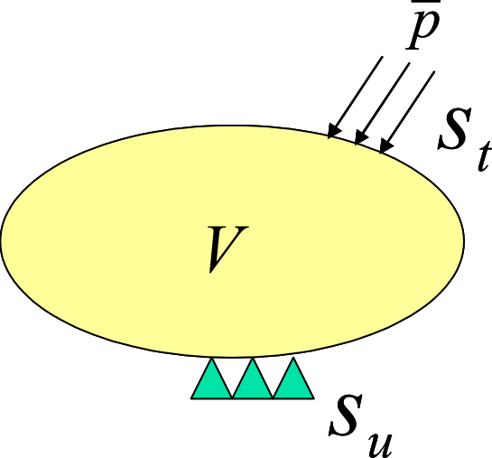
Figure 2.1.1 Boundary-value problem in solid mechanics (infinitesimal-deformation problem)

Using the symmetric gradient operator, the strain-displacement relation is

\[\begin{equation} \boldsymbol{\varepsilon} = \nabla_S \boldsymbol{u} \label{eq:2.1.4} \end{equation}\]

The linear-elastic constitutive equation is

\[\begin{equation} \boldsymbol{\sigma} = \boldsymbol{C} : \boldsymbol{\varepsilon} \label{eq:2.1.5} \end{equation}\]

where \(\boldsymbol{C}\) is the fourth-order elasticity tensor.

Principle of Virtual Work

The general forms of the principle of virtual work (current-configuration form, initial-configuration form, and reduction to infinitesimal deformation) are summarized in Principle of Virtual Work. Under the assumptions of infinitesimal deformation and linear elasticity, the weak form is

\[\begin{equation} \int_V \boldsymbol{\sigma} : \delta \boldsymbol{\varepsilon}\, dV = \int_{S_t} \overline{\boldsymbol{t}} \cdot \delta \boldsymbol{u}\, dS + \int_V \overline{\boldsymbol{b}} \cdot \delta \boldsymbol{u}\, dV \label{eq:2.1.6} \end{equation}\]

\[\begin{equation} \delta \boldsymbol{u} = \boldsymbol{0} \quad \text{on} \ S_u \label{eq:2.1.7} \end{equation}\]

Substituting the constitutive equation \eqref{eq:2.1.5} and writing \(\hat{\sigma} = D\, \hat{\varepsilon}\) in Voigt notation gives the form used directly for discretization:

\[\begin{equation} \int_V \delta \hat{\varepsilon}^T\, D\, \hat{\varepsilon}\, dV = \int_{S_t} \delta \boldsymbol{u}^T\, \overline{\boldsymbol{t}}\, dS + \int_V \delta \boldsymbol{u}^T\, \overline{\boldsymbol{b}}\, dV \label{eq:2.1.10} \end{equation}\]

is obtained, where \(D\) is the elastic matrix defined in Linear Elasticity. Equations \eqref{eq:2.1.10} and \eqref{eq:2.1.7} constitute the principle of virtual work discretized below.

Discretization and Assembly of the Global Equation

Discretizing the principle of virtual work in Eq.\( \eqref{eq:2.1.10} \) over the finite elements gives

\[\begin{equation} \sum_e \int_{V^e} \delta \hat{\varepsilon}^T\, D\, \hat{\varepsilon}\, dV = \sum_e \int_{S^e_t} \delta \boldsymbol{u}^T\, \overline{\boldsymbol{t}}\, dS + \sum_e \int_{V^e} \delta \boldsymbol{u}^T\, \overline{\boldsymbol{b}}\, dV \label{eq:2.1.11} \end{equation}\]

For each element, the displacement field is interpolated using the displacements of the nodes composing the element as follows.

\[\begin{equation} \boldsymbol{u} = \sum^m_{i=1} N_i\, \boldsymbol{u}_i = \boldsymbol{N}\, \boldsymbol{U} \label{eq:2.1.12} \end{equation}\]

The strain is then given using Eq.\(\eqref{eq:2.1.4}\) as follows.

\[\begin{equation} \hat{\varepsilon} = \boldsymbol{B}\, \boldsymbol{U} \label{eq:2.1.13} \end{equation}\]

Substituting Eqs.\(\eqref{eq:2.1.12}\) and \(\eqref{eq:2.1.13}\) into Eq.\(\eqref{eq:2.1.11}\) gives

\[\begin{equation} \sum_e \delta \boldsymbol{U}^T \left( \int_{V^e} \boldsymbol{B}^T D\, \boldsymbol{B}\, dV \right) \boldsymbol{U} = \sum_e \delta \boldsymbol{U}^T \int_{S_t^e} \boldsymbol{N}^T\, \overline{\boldsymbol{t}}\, dS + \sum_e \delta \boldsymbol{U}^T \int_{V^e} \boldsymbol{N}^T\, \overline{\boldsymbol{b}}\, dV \label{eq:2.1.14} \end{equation}\]

Equation \(\eqref{eq:2.1.14}\) can be written as

\[\begin{equation} \delta \boldsymbol{U}^T\, \boldsymbol{K}\, \boldsymbol{U} = \delta \boldsymbol{U}^T\, \boldsymbol{F} \label{eq:2.1.15} \end{equation}\]

Here, the components of the matrix and vector defined by Eqs.\(\eqref{eq:2.1.16}\) and \(\eqref{eq:2.1.17}\) can be calculated for each finite element and assembled by superposition.

\[\begin{equation} \boldsymbol{K} = \sum_e \int_{V^e} \boldsymbol{B}^T\, D\, \boldsymbol{B}\, dV \label{eq:2.1.16} \end{equation}\]

\[\begin{equation} \boldsymbol{F} = \sum_e \left( \int_{S_t^e} \boldsymbol{N}^T\, \overline{\boldsymbol{t}}\, dS + \int_{V^e} \boldsymbol{N}^T\, \overline{\boldsymbol{b}}\, dV \right) \label{eq:2.1.17} \end{equation}\]

Because Eq.\(\eqref{eq:2.1.15}\) holds for an arbitrary virtual displacement \(\delta \boldsymbol{U}\), the following equation is obtained.

\[\begin{equation} \boldsymbol{K}\, \boldsymbol{U} = \boldsymbol{F} \label{eq:2.1.18} \end{equation}\]

Meanwhile, the displacement boundary condition in Eq.\(\eqref{eq:2.1.3}\) is expressed as follows.

\[\begin{equation} \boldsymbol{U} = \overline{\boldsymbol{U}} \label{eq:2.1.19} \end{equation}\]

By solving Eq.\(\eqref{eq:2.1.18}\) subject to the constraint condition in Eq.\(\eqref{eq:2.1.19}\), the nodal displacement \(\boldsymbol{U}\) can be determined.

See Also